Parameter Estimation

In this section, we show how the BS-Warp and the NURBS-Warp parameters can be estimated. Here, we consider the feature-based approach for estimating the warp parameters. It has the advantage of being one of the most simple approach to estimate the parameters. We can thus concentrate on the main topic of this chapter, i.e. the representational power of the warps. As it was explained in section 5.1, this feature-based approach to image registration amounts to solve the following minimization problem:

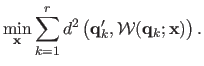$$\min_{\mathbf{x}} \sum_{k=1}^r d^2 \left ( \mathbf{q}'_k, \mathcal {W}(\mathbf{q}_k ; \mathbf{x}) \right ).$$ (6.13)

The main difficulty here is that problem (6.13) is not linear when using the NURBS-warps.

The BS-Warp

The dependency of the BS-Warp to its parameters is linear. As a consequence, the optimization problem (6.13) for a BS-Warp simply reduces to an ordinary linear least-squares minimization problem. The details for solving such a problem have already been detailed in, for instance, section 5.3.

The NURBS-Warp

Contrarily to the BS-Warp, the dependency of the NURBS-Warp to its parameters is not linear. Problem (6.13) thus leads one to a non-linear least-squares optimization problem. Note that this remark would still be true for other estimation techniques such as the direct approach to image registration. It is a well-known fact that this kind of problem can be efficiently solved using an iterative algorithm such as Levenberg-Marquardt. Such an algorithm needs an initial solution (see section 2.2.2.7). We propose three approaches to compute an initial set of parameters (which are further detailed in the sequel of this section):

• First approach: Act as if the images were taken under affine imaging conditions.
• Second approach: Act as if the warp relating the two images was an homography.
• Third approach: Use an algebraic approximation to the transfer error function.

Since all of these three approaches are relatively cheap to compute, it is possible to test the three of them and choose as initial parameters those that give the smallest transfer error.

First approach (affine initialization).

An initial solution for the NURBS-Warp estimation problem can be computed by setting all the weights to 1. By doing so, the equation defining a NURBS-warp reduces to the expression of a simple BS-Warp. An initial set of parameters can thus be computed using ordinary least-squares minimization. Since the BS-Warp corresponds to affine imaging conditions, this approach is expected to give good results when the effects of perspective are limited.

Second approach (homographic warp).

Even if the homographic warp is not suited to deformable environments, it can be a good approximation (particularly if the surface bending is not important). We denote  $\mathcal {W}_H$ the homographic warp. It is defined by:

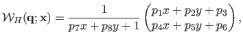$$\mathcal {W}_H(\mathbf{q} ; \mathbf{x}) = \frac{1}{p_7 x + p_8 y ... ...egin{pmatrix} p_1 x + p_2 y + p_3 p_4 x + p_5 y + p_6 \end{pmatrix},$$ (6.14)

with 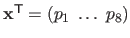 $\mathbf{x}^\mathsf{T}= (p_1 \; \ldots \; p_8)$. Minimizing the transfer error of equation (6.13) with the homographic warp  $\mathcal {W}_H$ can be achieved iteratively using, for instance, the Levenberg-Marquardt algorithm (and by taking the identity warp or the algebraic solution as an initialization). A complete review of homographic warp estimation can be found in (94).

Third approach (algebraic approximation).

The third and last approach we propose to initialize the optimization process consists in minimizing an algebraic approximation to the transfer error:

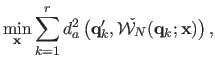$$\min_{\mathbf{x}} \sum_{k=1}^r d_a^2 \left( \mathbf{q}'_k, \check{\mathcal {W}_N}(\mathbf{q}_k ; \mathbf{x}) \right),$$ (6.15)

with $d_a^2\left( \mathbf{q}' , \check{\mathbf{q}} \right) = \left\Vert \mathsf{S} ( \tilde{\mathbf{q}}' \times \check{\mathbf{q}} ) \right\Vert^2$ an algebraic distance between the points^6.1  $\mathbf{q}$ and  $\mathbf{q}'$. The operator  $\mathsf{S}$ removes the last element of a 3-vector. $\tilde{\mathbf{q}}'$ are the scaled homogeneous coordinates of  $\mathbf{q}'$ (i.e. $\tilde{\mathbf{q}}'{}^\mathsf{T}= (\mathbf{q}'{}^\mathsf{T}\; 1)$). If we make the following variable change in equation (6.12) of the homogeneous NURBS-Warp: $a_{i,j} = p_{i,j}^x w_{i,j}$ and $b_{i,j}=p_{i,j}^y w_{i,j}$ then it is straightforward to see that the algebraic distance is the squared euclidean norm of an expression linear with respect to the parameters $a_{i,j}$, $b_{i,j}$ and $w_{i,j}$. Replacing the algebraic distance by its expression in the initial optimization problem of equation (6.15) leads to homogeneous linear least-squares. This problem can be solved using the singular value decomposition presented in section 2.2.2.10.