BleamCard: the first augmented reality card. Get your own on Indiegogo!
Subsections
Basics on Continuous Optimization
Most of the problems solved in this thesis can be formulated as optimization problems.
In this section, we give some general points on optimization.
We also give details on the most used optimization algorithms in this document.
The statistical grounds of certain type of cost function will be explained in section 3.1.
In its general form, an unconstrained minimization problem has the following form (25,52,154,136,22):
 |
(2.17) |
The function  is a scalar-valued function named the cost function or the criterion.
It is assumed that the cost function is defined on
is a scalar-valued function named the cost function or the criterion.
It is assumed that the cost function is defined on
 .
In some cases later explained, can be a vector-valued function instead of a scalar-valued one.
Note that we only consider the case of the minimization of the cost function since the problem of maximization can easily be turned into a minimization problem (by taking the negative of the cost function).
.
In some cases later explained, can be a vector-valued function instead of a scalar-valued one.
Note that we only consider the case of the minimization of the cost function since the problem of maximization can easily be turned into a minimization problem (by taking the negative of the cost function).
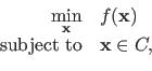
A constrained minimization problem is similar to an unconstrained minimization problem except that supplemental conditions on the solution must be satisfied.
Such a problem has the following form:
 |
(2.18) |
where  is a set defining the constraints.
These constraints can take many forms.
For instance, it can be inequality constraints such as
is a set defining the constraints.
These constraints can take many forms.
For instance, it can be inequality constraints such as
 , linear equality constraints such as
 for some matrix
 and some vector
 .
It can also be more complex constraints such as
.
It can also be more complex constraints such as
 where
where  is some function.
These are just a few examples.
is some function.
These are just a few examples.
In this section we focus on unconstrained minimization problem since it is the main tool used in this thesis.
An optimization algorithm is an algorithm that provides a solution to an optimization problem.
There exists a vast amount of optimization algorithms.
The algorithm used to solve an optimization problem depends on the properties of the cost function and of the constraints.
For instance, the optimization algorithm depends on the differentiability of the cost function.
It can also exploit a particular form of the cost function (for instance, a cost function defined as a sum of squares).
The ultimate goal of a minimization problem is to find a global minimum of the cost function, i.e. a vector
 such that:
 |
(2.19) |
The solutions proposed by optimization algorithms are only guaranteed to be local minima.
A vector
 is said to be a local minimizer of the function if the following statement is true:
 |
(2.20) |
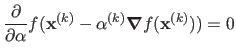
When the function is differentiable, a necessary condition for
to be a local minimizer is:
 |
(2.21) |
A local minimum of the function is not necessarily a global minimum of the function.
Indeed, a cost function may have several local minima.
Deciding whether a local minima is a global minimum or not is an undecidable problem.
Convexity is a particularly interesting property for a function.
Indeed, if a cost function is convex then it has only one minimum which is therefore a global minimum of the function.
Note that the converse is not true; there exist non-convex functions which have only one (global) minimum.
Let
 be a scalar-valued function.
Let
be a scalar-valued function.
Let
 and
and
 .
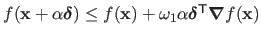
A scalar function is said to be convex if the following condition holds for all
.
A scalar function is said to be convex if the following condition holds for all
![$ \alpha \in [0,1]$](img141.png) :
:
 |
(2.22) |
Alternatively, if the function is twice differentiable, then is convex if the Hessian matrix
 is positive definite.
A strictly convex function is a function that satisfies equation (2.22) with the  sign replaced by
  .
Note that the Hessian matrix of a twice differentiable strictly convex function is not necessarily strictly positive definite: it might only be positive definite.
.
Note that the Hessian matrix of a twice differentiable strictly convex function is not necessarily strictly positive definite: it might only be positive definite.
Optimization Algorithms
In this section, we present the unconstrained minimization algorithms mostly used in this thesis.
The choice of an optimization algorithm depends on the properties of the cost function to be minimized.
These algorithms can be classified according to several criterion.
Table 2.1 summarizes the optimization algorithm reviewed in this section and the properties that must be satisfied by the cost function.
This section is organized as follows: we go from the less restrictive algorithms (in terms of conditions on the cost function) to most restrictive ones (i.e. the more specific).
Two sections not dedicated to a specific optimization algorithm are intercalated in this section: section 2.2.2.1 gives some general points on iterative optimization algorithms, and section 2.2.2.6 talks about the normal equations.
Table 2.1:
Optimization algorithms reviewed in section 2.2.2. They are ordered from the more generic to the less generic. `Abb.' in the second column stands for `Abbreviation'.
|
|
Iterative Optimization Algorithms
Before talking about the details, let us start with some generalities on the optimization algorithms.
Most of these algorithms are iterative algorithms.
This means that they start from an initial value
 which is then iteratively updated.
Therefore, an iterative optimization algorithm builds a sequence
which is then iteratively updated.
Therefore, an iterative optimization algorithm builds a sequence
 that may converge towards a local minimum of the cost function, i.e.
 may be close to a local minimum of the solution.
With a cost function that has several minima, the initial value
determines which minimum is found.
This initial value is thus extremely important.
may be close to a local minimum of the solution.
With a cost function that has several minima, the initial value
determines which minimum is found.
This initial value is thus extremely important.
An important aspect of iterative optimization algorithm is the stopping criterion.
For the algorithm to be valid, the stopping criterion must be a condition that will be satisfied in a finite and reasonable amount of time.
A stopping criterion is usually the combination of several conditions.
For instance, one can decide to stop the algorithm when the change in the solution becomes very small, i.e. when
 with
with
 a small fixed constant (for instance,
 ).
Of course, this approach does not account for the scale of the solution.
One may replace this condition using, for instance, a relative change, i.e.
).
Of course, this approach does not account for the scale of the solution.
One may replace this condition using, for instance, a relative change, i.e.
 .
Another standard stopping criterion is the change in the cost function value:
.
Another standard stopping criterion is the change in the cost function value:
 .
A maximal number of iterations must also be determined to guarantee that the optimization algorithm will finish in a finite amount of time.
Indeed, the previous two stopping criterion may never be satisfied.
In the rest of this section, we will denote STOP-CRIT the stopping criterion.
In addition to what was just presented, the content of STOP-CRIT will be further detailed depending on the optimization algorithm.
.
A maximal number of iterations must also be determined to guarantee that the optimization algorithm will finish in a finite amount of time.
Indeed, the previous two stopping criterion may never be satisfied.
In the rest of this section, we will denote STOP-CRIT the stopping criterion.
In addition to what was just presented, the content of STOP-CRIT will be further detailed depending on the optimization algorithm.
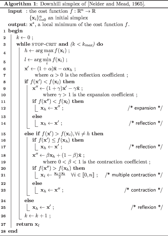
Downhill Simplex
The downhill simplex method is an optimization algorithm due to (134).
It is a heuristic that does not make any assumption on the cost function to minimize.
In particular, the cost function must not satisfy any condition of differentiability.
It relies on the use of simplices, i.e. polytopes of dimension  .
For instance, in two dimensions, a simplex is a polytope with 3 vertices, most commonly known as a triangle.
In three dimensions, a simplex is tetrahedron.
.
For instance, in two dimensions, a simplex is a polytope with 3 vertices, most commonly known as a triangle.
In three dimensions, a simplex is tetrahedron.
We now explain the mechanisms of the downhill simplex method of (134).
Note that more sophisticated versions of this method have been proposed.
This is the case, for instance, of the algorithm used by the fminsearch function of Matlab.
The downhill simplex method starts from an initial simplex.
Each step of the method consists in an update of the current simplex.
These updates are carried out using four operations: reflection, expansion, contraction, and multiple contraction.
Let
 be the function to minimize and let
 be the current simplex (
 for all
 ).
Let
).
Let
 be the index of the `worst vertex', i.e. the value
 and let
 be the index of the `best vertex', i.e. the value
 .
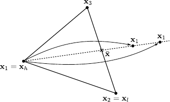
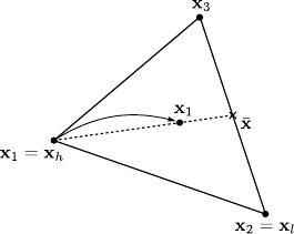
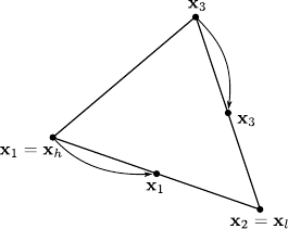
The downhill simplex method and the four fundamental operations are detailed in algorithm 1.
Figure 2.1 illustrates the four fundamental operations on a 3-simplex.
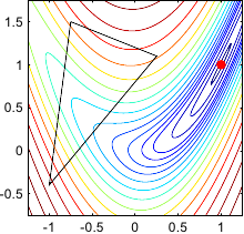
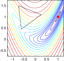
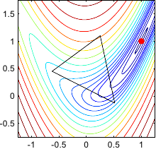
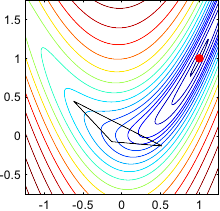
In figure 2.3, as an example, the downhill simplex method is used to optimize the Rosenbrock function (see below).
.
The downhill simplex method and the four fundamental operations are detailed in algorithm 1.
Figure 2.1 illustrates the four fundamental operations on a 3-simplex.
In figure 2.3, as an example, the downhill simplex method is used to optimize the Rosenbrock function (see below).
Figure 2.1:
Illustration in 2 dimensions of the four fundamental operations applied to the current simplex by the downhill simplex method of (134): (a) reflection and expansion, (b) contraction, and (c) multiple contraction.
|
|
The stopping criterion used by (134) is defined by:
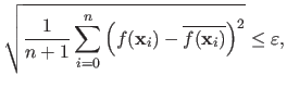 |
(2.23) |
with
 the average of the values
 , and
a predefined constant.
This criterion has the advantage of linking the size of the simplex with an approximation of the local curvature of the cost function.
A very accurate minimum is often obtained for a high curvature of the cost function.
On the contrary, a minimum located in a flat valley of the cost function carries less information.
Therefore, it does not make much sense to shrink an optimal simplex which would be almost flat.
, and
a predefined constant.
This criterion has the advantage of linking the size of the simplex with an approximation of the local curvature of the cost function.
A very accurate minimum is often obtained for a high curvature of the cost function.
On the contrary, a minimum located in a flat valley of the cost function carries less information.
Therefore, it does not make much sense to shrink an optimal simplex which would be almost flat.
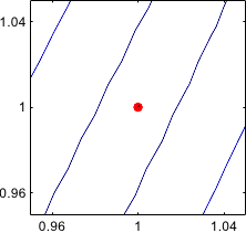
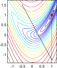
When it is possible, the algorithms presented in this section are illustrated on the Rosenbrock function.
This function, also known as the banana function, has been a standard test case for optimization algorithms.
It is a two-dimensional function defined as:
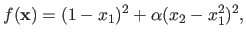 |
(2.24) |
with  a positive constant.
In our illustrations, we use
a positive constant.
In our illustrations, we use
 .
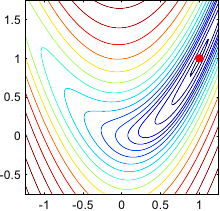
The minimum is inside a long, narrow, parabolic flat valley.
Finding the valley is simple but finding the actual minimum of the function is less trivial.
The minimum of the Rosenbrock function is located at the point of coordinate
.
The minimum is inside a long, narrow, parabolic flat valley.
Finding the valley is simple but finding the actual minimum of the function is less trivial.
The minimum of the Rosenbrock function is located at the point of coordinate
 , whatever the value given to .
Figure 2.2 gives an illustration of this function.
, whatever the value given to .
Figure 2.2 gives an illustration of this function.
Figure 2.2:
Contour plot of the Rosenbrock banana function.
|
 |
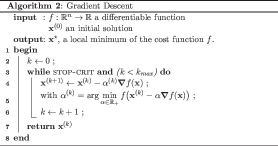
Gradient descent
The method of gradient descent (also known as the method of steepest descent or Cauchy's method) is one the most simple algorithm for continuous optimization (52).
It was first designed to solve linear system a long time ago (43).
It is an iterative algorithm that relies on the fact that the value of the cost function decreases fastest in the direction of the negative gradient (for a differentiable cost function).
The principle of the gradient descent algorithm is given in algorithm 2.
The exact line search procedure of line 5 in algorithm 2 can be replaced with an approximate line search procedure such that the value
 satisfies the Wolfe conditions (136,126) (see below).
As a first remark, we can notice that the successive search directions used by the gradient descent method are always orthogonal to the level sets of the cost functions.
Second, we may also notice that if an exact line search procedure is used, then the method of gradient descent is guaranteed to converge to a local minimum.
Under some mild assumptions, it has also been proven to converge with an inexact line search procedure (see, for instance, (40)).
However, this convergence is usually very slow.
This stems from the fact that, if an exact line search procedure is used, two successive directions are necessarily orthogonal.
This is easy to see.
Indeed, if
minimizes
 then we have:
which proves that the search directions at iteration  and
and  are orthogonal.
Therefore, the path formed by the values
are orthogonal.
Therefore, the path formed by the values
 is shaped like a stairs.
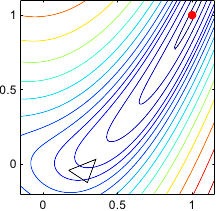
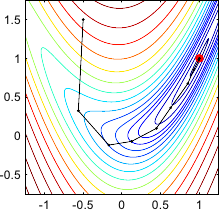
Figure 2.4 gives an illustration on the Rosenbrock function of this typical behaviour of the gradient descent method.
is shaped like a stairs.
Figure 2.4 gives an illustration on the Rosenbrock function of this typical behaviour of the gradient descent method.
Figure 2.4:
Illustration of the successive steps taken by the method of the gradient descent for optimizing the Rosenbrock functions. Notice that the successive search directions are orthogonal. In (b), we see the typical stair effect of this method. It makes the convergence very slow. Indeed, after 100 iterations, convergence has not yet been reached.
|
 |
 |
| (a) |
(b) |
|
Given a search direction
 , an exact line search procedure amounts to solve the following mono-dimensional minimization problem:
 |
(2.28) |
Problem (2.28) can be solved using an algorithm such as the golden section search that will be presented in section 2.2.2.12.
Depending on the function , problem (2.28) can be heavy to compute.
Another approach consists in doing an approximate line search.
It consists in starting from an initial estimate of and then refine it so that the Wolfe conditions are satisfied.
The Wolfe conditions gives some criteria to decide whether a step is satisfactory or not.
In its basic form, there are two Wolfe conditions:
-
-
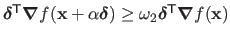
with  and
and  two constants such that
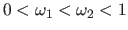 . is usually chosen as a small constant and as a constant (much) bigger than .
The first condition (also known as the Armijo condition) avoids long steps that would not decrease much the cost function.
The second condition (also known as the curvature condition) forces the step to minimize the curvature of the cost function.
. is usually chosen as a small constant and as a constant (much) bigger than .
The first condition (also known as the Armijo condition) avoids long steps that would not decrease much the cost function.
The second condition (also known as the curvature condition) forces the step to minimize the curvature of the cost function.
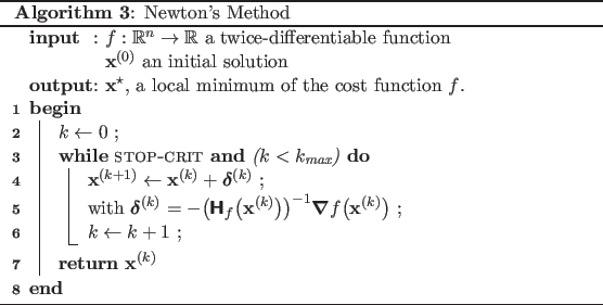
Newton's Method
Newton's method is another iterative optimization algorithm that minimizes a twice-differentiable function
.
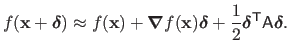
It relies on the second order Taylor expansion of the function around the point
:
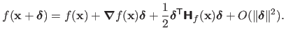 |
(2.29) |
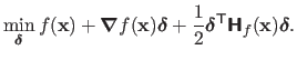
Each step of the Newton's method consists in finding the minimum of the quadratic approximation of the function around the current point
.
This principle can be stated using the second order Taylor expansion of :
 |
(2.30) |
A necessary condition for problem (2.30) is obtained by setting to zero the derivative (with respect to
) of the cost function in equation (2.30).
This amounts to solve the following linear system of equations:
 |
(2.31) |
The search direction
for the Newton method is thus given by:
 |
(2.32) |
Note that, in practice, the inverse Hessian matrix in equation (2.32) does not need to be explicitly calculated ;
it is possible to compute
from equation (2.31) using an efficient solver of linear systems.
The complete Newton's method is summarized in algorithm 3.
Algorithm 3 is the constant step version of Newton's algorithm.
The update
 is often replaced by the update
 where
where  is a positive value smaller than 1.
This is done to insure that the Wolfe conditions are satisfied for each step of the algorithm.
is a positive value smaller than 1.
This is done to insure that the Wolfe conditions are satisfied for each step of the algorithm.
Every local minimum of the function has a neighbourhood  in which the convergence of Newton's method with constant step is quadratic (52).
In other words, if we initialize the Newton's method with
in which the convergence of Newton's method with constant step is quadratic (52).
In other words, if we initialize the Newton's method with
 , the convergence is quadratic.
Outside of the neighbourhoods of the local minima of the cost function, there are no guarantee that Newton's method will converge.
Indeed the condition of equation (2.31) is just a necessary condition for having a local minimum: it is not a sufficient condition.
The condition of equation (2.31) is also satisfied for a local maximum or a saddle point of the cost function.
Therefore, Newton's method can converge towards such points.
, the convergence is quadratic.
Outside of the neighbourhoods of the local minima of the cost function, there are no guarantee that Newton's method will converge.
Indeed the condition of equation (2.31) is just a necessary condition for having a local minimum: it is not a sufficient condition.
The condition of equation (2.31) is also satisfied for a local maximum or a saddle point of the cost function.
Therefore, Newton's method can converge towards such points.
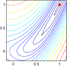
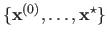
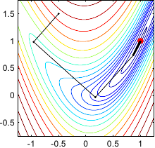
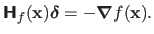
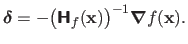
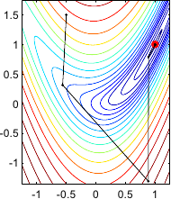
An illustration of Newton's method on the Rosenbrock function is given in figure 2.5.
Two variants are presented in this figure: the constant step length variant and the optimal step length determined with a line search strategy.
Figure 2.5:
Illustration of the successive steps taken by Newton's method for optimizing the Rosenbrock functions. (a) Constant step length variant. (b) Step length determined with an optimal line search strategy. On the Rosenbrock function, the Newton method is usually faster to converge than the gradient descent strategy. In this particular example, convergence is reached within 6 iterations for the constant step length variant and 10 iterations with the optimal line search strategy.
|
 |
 |
| (a) |
(b) |
|
Newton's method is great since it usually converges quickly.
This means that it does not take a lot of iterations to reach the minimum.
However, each iteration of this algorithm can be costly since it requires one to compute the Hessian matrix.
The goal of quasi-Newton approach is to replace the Hessian matrix by some good approximation, less heavy to compute.
There exists several formula to make these approximations iteratively: DFP, SR1, BFGS (52).
We will not detail these formula here but we will give the general principle.
As for Newton's method, quasi-Newton relies on the second order Taylor expansion of the function to optimize, except that the Hessian matrix is replaced with an approximation
:
 |
(2.33) |
The gradient of this approximation with respect to
is given by:
 |
(2.34) |
The general principle of a quasi-Newton approach is to choose the matrix
such that:
 |
(2.35) |
The difference between the different formula are the properties that the matrix
satisfies at each iteration of the algorithm.
For instance, the BFGS method guarantees that the matrix
will always be symmetric and positive definite.
In this case, the approximation of the cost function is convex and, therefore, the search direction is guaranteed to be a descent direction.
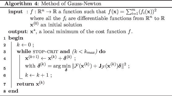
Gauss-Newton Algorithm
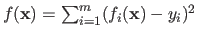
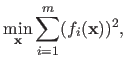
The Gauss-Newton method is an optimization algorithm used to minimize a cost function that can be written as a sum of squares, i.e. if
:
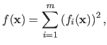 |
(2.36) |
where each  for
for
 is a function of the form
 .
The only hypothesis that must be satisfied for the Gauss-Newton algorithm is that the functions must all be differentiable.
Equation (2.36) is the very definition of a least-squares problem.
For reasons that will become clear in the next section, least-squares cost functions often arises when estimating the parameters of a parametric model.
The derivation of the Gauss-Newton algorithm is more conveniently done if we consider the minimization of a vector-valued function
.
The only hypothesis that must be satisfied for the Gauss-Newton algorithm is that the functions must all be differentiable.
Equation (2.36) is the very definition of a least-squares problem.
For reasons that will become clear in the next section, least-squares cost functions often arises when estimating the parameters of a parametric model.
The derivation of the Gauss-Newton algorithm is more conveniently done if we consider the minimization of a vector-valued function
 :
:
 |
(2.37) |
where
 is defined as:
 |
(2.38) |
Note that solving problem (2.37) is completely equivalent to minimizing the function as defined in equation (2.36).
The Gauss-Newton algorithm is an iterative algorithm where each step consists in minimizing the first-order approximation of the function
around the current solution.
The first-order approximation of
is given by:
 |
(2.39) |
Therefore, each step of the Gauss-Newton algorithm consists in determining the step
by solving the following minimization problem:
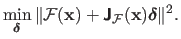 |
(2.40) |
Problem (2.40) is a linear least-squares minimization problem.
As it will be seen later, such a problem can easily be solved.
Algorithm 4 gives the complete principle of the Gauss-Newton method.
As for the others algorithms presented so far, a line-search procedure can be combined to the step.
It can be shown that the step
is a descent direction (22).
If the algorithm converges then the limit is a stationary point of the function (but not necessarily a minimum).
However, with no assumptions on the initial solution, there is no guarantee that the algorithm will converge, even locally.
With a good starting point and a `nice' function (i.e. a mildly nonlinear function), the convergence speed of the Gauss-Newton method is almost quadratic.
However, it can be worse than quadratic if the starting point is far from the minimum or if the matrix
 is ill-conditioned.
The Rosenbrock function can be written as a sum of squares if we define the functions  and
and  in the following way:
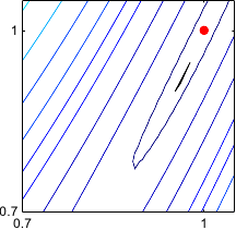
Figure 2.6 shows the step taken by the Gauss-Newton algorithm for minimizing the Rosenbrock function.
Figure 2.6:
Illustration of the Gauss-Newton method on the Rosenbrock function. For this simple example, the optimal solution is found in 2 iterations.
|
 |
The Normal Equations
We broke a little bit our classification of the optimization algorithms and present now a basic tool for linear least-squares problems: the normal equations.
We do so because, as it was just seen, the iterations of the Gauss-Newton algorithm involves the solution of a linear least-squares minimization problem.
Besides, a part of the algorithm we present next, namely the Levenberg-Marquardt algorithm, uses the so-called normal equations.
Let
be the function to minimize.
Let us suppose that can be written as a sum of squares of the form
 , where the functions
 are linear with respect to
(i.e.
are linear with respect to
(i.e.
 such that
 , for all
) and where
, for all
) and where
 for all
.
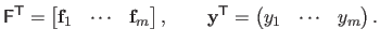
Minimizing the function can be stated in matrix form:
for all
.
Minimizing the function can be stated in matrix form:
 |
(2.43) |
where the matrix
 and the vector
 are defined by:
 |
(2.44) |
If the matrix
 has full column rank (22), problem (2.43) can be solved using the normal equations:
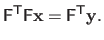 |
(2.45) |
The hypothesis that
has full column rank allows us to say that the square matrix
 is invertible.
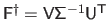
The solution of problem (2.45) (and therefore of problem (2.43)) is given by:
is invertible.
The solution of problem (2.45) (and therefore of problem (2.43)) is given by:
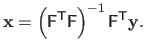 |
(2.46) |
Since the matrix
 has full column rank, it is the Moore-Penrose pseudo-inverse matrix of
and is denoted
has full column rank, it is the Moore-Penrose pseudo-inverse matrix of
and is denoted
 .
It is generally a bad practice to explicitly compute the pseudo-inverse matrix (83).
We will see later in this document several methods designed to efficiently solve the linear system of equation (2.45).
Note that
being full column rank necessary implies that
must have more rows than columns, i.e.
.
It is generally a bad practice to explicitly compute the pseudo-inverse matrix (83).
We will see later in this document several methods designed to efficiently solve the linear system of equation (2.45).
Note that
being full column rank necessary implies that
must have more rows than columns, i.e.  .
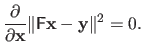
There exists several ways to derive the normal equations.
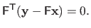
For instance, one can get them by writing the optimality conditions of problem (2.43), i.e. :
.
There exists several ways to derive the normal equations.
For instance, one can get them by writing the optimality conditions of problem (2.43), i.e. :
 |
(2.47) |
The normal equations are trivially derived by noticing that
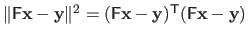 .
Another way to obtain the normal equations is to consider the over-determined linear system of equations:
.
Another way to obtain the normal equations is to consider the over-determined linear system of equations:
 |
(2.48) |
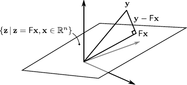
Since this linear system of equations is over-determined, it does not have necessarily an exact solution.
In this case, we can seek for an approximate solution by finding the point of the column space of
which is as close as possible to the point
 .
The shortest distance between a point and an hyperplane is the distance between the point and its orthogonal projection into the hyperplane.
This is illustrated by figure 2.7.
In other words, the vector
.
The shortest distance between a point and an hyperplane is the distance between the point and its orthogonal projection into the hyperplane.
This is illustrated by figure 2.7.
In other words, the vector
 must lie in the left nullspace of
, which can be written:
must lie in the left nullspace of
, which can be written:
 |
(2.49) |
Equation (2.49) are exactly equivalent to the normal equations.
Figure 2.7:
Graphical interpretation of the normal equations.
|
 |
Levenberg-Marquardt
The Levenberg algorithm is another method to solve a least-squares minimization problem proposed by (110).
(121) proposed a slight variation of the initial method of Levenberg known as the Levenberg-Marquardt algorithm.
The content and the presentation of this section is inspired by (117).
We use the same notation than in the section dedicated to the Gauss-Newton algorithm.
The normal equations can be used for the step in the Gauss-Newton algorithm.
This step, denoted
 in this section, can thus be written
 , where
 is the Jacobian matrix of the function
evaluated at
, and
is the Jacobian matrix of the function
evaluated at
, and
 .
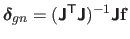
The Levenberg and the Levenberg-Marquardt algorithms are damped versions of the Gauss-Newton method.
The step for the Levenberg algorithm, denoted
.
The Levenberg and the Levenberg-Marquardt algorithms are damped versions of the Gauss-Newton method.
The step for the Levenberg algorithm, denoted
 , is defined as:
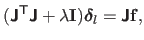 |
(2.50) |
while the step for the Levenberg-Marquardt algorithm, denoted
 , is defined as:
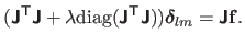 |
(2.51) |
From now on, we only consider the Levenberg-Marquardt algorithm2.2.
The linear system of equation (2.51) is called the augmented normal equations.
The value  is a positive value named the damping parameter.
It plays several roles.
First, the matrix
is a positive value named the damping parameter.
It plays several roles.
First, the matrix
 is positive definite.
Therefore,
is necessarily a descent direction.
For large values of ,
is positive definite.
Therefore,
is necessarily a descent direction.
For large values of ,
 .
In this case, the Levenberg-Marquardt algorithm is almost a gradient descent method (with a short step).
This is a good strategy when the current solution is far from the minimum.
On the contrary, if is a small value, then the Levenberg-Marquardt step
is almost identical to the Gauss-Newton step
.
This is a desired behaviour for the final steps of the algorithm since, near the minimum, the convergence of the Gauss-Newton method can be almost quadratic.
.
In this case, the Levenberg-Marquardt algorithm is almost a gradient descent method (with a short step).
This is a good strategy when the current solution is far from the minimum.
On the contrary, if is a small value, then the Levenberg-Marquardt step
is almost identical to the Gauss-Newton step
.
This is a desired behaviour for the final steps of the algorithm since, near the minimum, the convergence of the Gauss-Newton method can be almost quadratic.
Both the length and the direction of the step are influenced by the damping parameter.
Consequently, there is no need for a line-search procedure in the iterations of this algorithm.
The value of the damping parameter is updated along with the iterations according to the following strategy.
If the current results in an improvement of the cost function, then the step is applied and is divided by a constant  (with, typically,
  ).
On the contrary, if the step resulting of the current increases of the function, the step is discarded and is multiplied by .
This is the most basic stratagem for updating the damping parameter.
There exists more evolved approach, such as the one presented in (117).
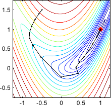
The whole Levenberg-Marquardt method is given in algorithm 5.
Figure 2.8 gives an illustration of the Levenberg-Marquardt algorithm on the Rosenbrock function.
).
On the contrary, if the step resulting of the current increases of the function, the step is discarded and is multiplied by .
This is the most basic stratagem for updating the damping parameter.
There exists more evolved approach, such as the one presented in (117).
The whole Levenberg-Marquardt method is given in algorithm 5.
Figure 2.8 gives an illustration of the Levenberg-Marquardt algorithm on the Rosenbrock function.
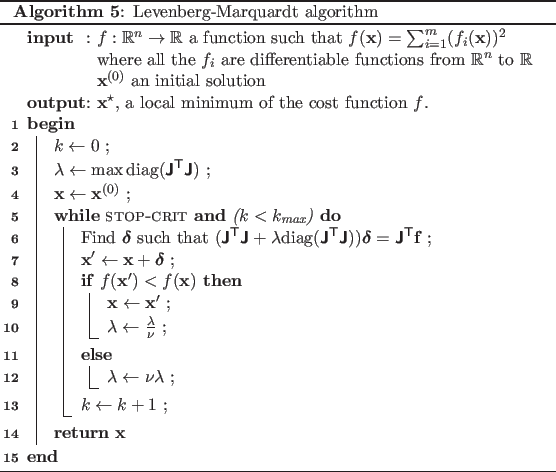
Figure 2.8:
Illustration of the Levenberg-Marquardt algorithm for optimizing the Rosenbrock function. In this particular example, this algorithm took 25 iterations to reach the minimum.
|
 |
Cholesky Factorization
We now provides some tools for solving efficiently a linear system of equations.
This is of great interest in optimization since we have seen that solving a linear least-squares minimization problem is equivalent to finding a solution to the linear system formed by the normal equations.
Besides, other optimization problems (not necessarily written as linear least-squares problem) involves a linear least-squares problem in their iterations.
Let us consider the following linear system of equations:
 |
(2.52) |
with
 a square matrix, and
 .
The problem equation (2.52) admits a single solution if the determinant of the matrix
is not null.
In this case, the solution is theoretically given with the inverse matrix of
, i.e.
.
The problem equation (2.52) admits a single solution if the determinant of the matrix
is not null.
In this case, the solution is theoretically given with the inverse matrix of
, i.e.
 .
However, explicitly forming the matrix
.
However, explicitly forming the matrix
 is generally not the best way of solving a linear system of equations (83).
This stems from the fact that a direct computation of the inverse matrix is numerically unstable.
Besides, it is not possible to exploit sparse properties of a matrix when explicitly forming the inverse matrix.
A very basic tool that can be used to solve a linear system is the Gauss elimination algorithm (154,83).
The main advantage of this algorithm is that it does not need strong assumption on the matrix of the system (except that it is square and invertible, of course).
Here, we will not give the details of the Gauss elimination algorithm.
Instead, we will present other algorithms more suited to the intended purpose, i.e. optimization algorithms.
is generally not the best way of solving a linear system of equations (83).
This stems from the fact that a direct computation of the inverse matrix is numerically unstable.
Besides, it is not possible to exploit sparse properties of a matrix when explicitly forming the inverse matrix.
A very basic tool that can be used to solve a linear system is the Gauss elimination algorithm (154,83).
The main advantage of this algorithm is that it does not need strong assumption on the matrix of the system (except that it is square and invertible, of course).
Here, we will not give the details of the Gauss elimination algorithm.
Instead, we will present other algorithms more suited to the intended purpose, i.e. optimization algorithms.
The Cholesky factorization is a method for solving a linear system of equations.
If the matrix
is positive definite, then the Cholesky factorization of
is:
 |
(2.53) |
with
 an upper triangular matrix with strictly positive diagonal entries.
Note that, for example, the left-hand side of the augmented normal equations used in the iterations of the Levenberg-Marquardt algorithm is a positive definite matrix.
If we substitute the matrix
in equation (2.52) by its Cholesky factorization, we obtain:
an upper triangular matrix with strictly positive diagonal entries.
Note that, for example, the left-hand side of the augmented normal equations used in the iterations of the Levenberg-Marquardt algorithm is a positive definite matrix.
If we substitute the matrix
in equation (2.52) by its Cholesky factorization, we obtain:
 |
(2.54) |
If we note
 then solving equation (2.52) is equivalent to successively solving the two linear systems
 and
and
 .
This is easily and efficiently done using a back-substitution process because of the triangularity of the matrices
.
This is easily and efficiently done using a back-substitution process because of the triangularity of the matrices
 and
and
 .
.
Although efficient, this approach works only if the problem is well-conditioned.
If not, some of the diagonal entries of the matrix
are close to zero and the back-substitution process becomes numerically unstable.
In practice, the Cholesky factorization is particularly interesting for sparse matrices.
For instance, the package cholmod of (55), dedicated to sparse matrices, heavily uses Cholesky factorization.
QR Factorization
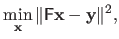
We now give a method based on the QR factorization for solving an over-determined linear least-squares minimization problem of the form:
|
(2.55) |
with
, , and
.
As we have seen in section 2.2.2.6, solving problem (2.55) amounts to solve the normal equations, namely:
|
(2.56) |
The QR factorization of the matrix
is:
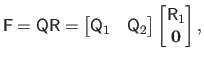 |
(2.57) |
with
 an orthonormal matrix,
 ,
,
 , and
, and
 an upper triangular matrix.
If the matrix
has full column rank, then the columns of the matrix
an upper triangular matrix.
If the matrix
has full column rank, then the columns of the matrix
 form an orthonormal basis for the range of
(84).
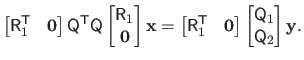
If we replace the matrix
by its QR factorization into the normal equations, we obtain:
form an orthonormal basis for the range of
(84).
If we replace the matrix
by its QR factorization into the normal equations, we obtain:
 |
(2.58) |
This last expression can be simplified using the fact that the matrix
is orthonormal:
 |
(2.59) |
As for the approach based on the Cholesky factorization, the linear system of equation (2.59) can be easily solved with a back-substitution algorithm.
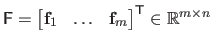
Singular Value Decomposition
The singular value decomposition is a tool that can be used to solve certain linear least-squares minimization problems.
The singular value decomposition of a real matrix
 is given by:
 |
(2.60) |
with
 a unitary matrix,
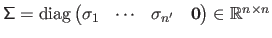
 a diagonal matrix with non-negative elements on its diagonal, and
 a unitary matrix.
The diagonal entries of
a unitary matrix.
The diagonal entries of
 , named the singular values, are generally sorted from the largest to the smallest.
If the matrix
has full column rank then the diagonal entries of
are all strictly positive.
In fact, the number of strictly positive elements on the diagonal of
is the rank of the matrix
.
, named the singular values, are generally sorted from the largest to the smallest.
If the matrix
has full column rank then the diagonal entries of
are all strictly positive.
In fact, the number of strictly positive elements on the diagonal of
is the rank of the matrix
.
Once again, we consider the problem of minimizing the over-determined linear least-squares function
 .
This least-squares problem is called non-homogeneous because there exists a non-null right-hand side
.
The singular value decomposition can be used to solve this problem.
Indeed, if we replace the matrix
in the normal equations by its singular value decomposition
.
This least-squares problem is called non-homogeneous because there exists a non-null right-hand side
.
The singular value decomposition can be used to solve this problem.
Indeed, if we replace the matrix
in the normal equations by its singular value decomposition
 , we obtain:
 |
(2.61) |
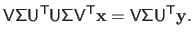
Using the fact that
 is a unitary matrix and that
is a diagonal matrix, we can write that:
is a unitary matrix and that
is a diagonal matrix, we can write that:
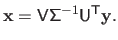 |
(2.62) |
In other words, we have that
 .
As for the other algorithms, the computational complexity of this method is in
.
As for the other algorithms, the computational complexity of this method is in
 .
The main advantage of the SVD approach for linear least-squares problem is when the matrix
is almost rank deficient.
In this case, the smallest singular values in
are very close to zero.
Therefore, a simple computation of
.
The main advantage of the SVD approach for linear least-squares problem is when the matrix
is almost rank deficient.
In this case, the smallest singular values in
are very close to zero.
Therefore, a simple computation of
 would lead to unsatisfactory results (the inverse of a diagonal matrix being obtained by taking the reciprocals of the diagonal entries of
).
In this case, one can replace the inverse matrix
in equation (2.62) by the pseudo-inverse matrix
would lead to unsatisfactory results (the inverse of a diagonal matrix being obtained by taking the reciprocals of the diagonal entries of
).
In this case, one can replace the inverse matrix
in equation (2.62) by the pseudo-inverse matrix
 .
The pseudo-inverse of a diagonal matrix
.
The pseudo-inverse of a diagonal matrix
 (with
(with  ) is the matrix
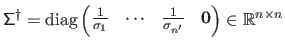 .
.
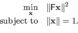
We now consider the case of the homogeneous linear least-squares minimization problem.
It corresponds to the following minimization problem:
 |
(2.63) |
where the functions
are linear with respect to
, i.e.
such that
for all
.
This minimization problem can be written in matrix form:
 |
(2.64) |
with
 .
An obvious solution to problem (2.64) is
.
An obvious solution to problem (2.64) is
 .
Of course, this dummy solution is generally not interesting.
Instead of solving problem (2.64), one replaces it with the following constrained optimization problem:
.
Of course, this dummy solution is generally not interesting.
Instead of solving problem (2.64), one replaces it with the following constrained optimization problem:
 |
(2.65) |
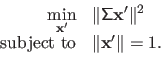
Problem (2.65) is easily solved using the singular value decomposition.
Indeed, let
be the singular value decomposition of
.
If we write
 , then problem (2.65) is equivalent to:
 |
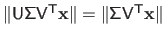
(2.66) |
This stems from the fact that the matrices
and
 are unitary and, consequently, we have that
 and
and
 .
Remind the fact that for a full column rank matrix the diagonal elements of
are
.
Remind the fact that for a full column rank matrix the diagonal elements of
are
 .
Therefore, an evident minimizer of problem (2.66) is
.
Therefore, an evident minimizer of problem (2.66) is
 .
Finally, since we have that
.
Finally, since we have that
 , the solution of our initial homogeneous linear least-squares problem is given by the last column of the matrix
.
If the matrix
has not full column rank, then the same principle can be applied except that one may take the column of
corresponding the last non-zero singular value.
, the solution of our initial homogeneous linear least-squares problem is given by the last column of the matrix
.
If the matrix
has not full column rank, then the same principle can be applied except that one may take the column of
corresponding the last non-zero singular value.
Iteratively Reweighed Least Squares
The method of Iteratively Reweighed Least Squares (IRLS) is an optimization algorithm designed to minimize a function
of the form:
 |
(2.67) |
where  is a function from
to
is a function from
to
 .
For instance, such a cost function arises when M-estimators are involved.
IRLS is an iterative method for which each step involves the resolution of the following weighted least squares problem:
.
For instance, such a cost function arises when M-estimators are involved.
IRLS is an iterative method for which each step involves the resolution of the following weighted least squares problem:
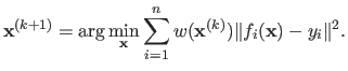 |
(2.68) |
Golden Section Search
We now arrive at the last optimization algorithm presented in this document: the golden section search algorithm.
This algorithm allows one to minimize a monovariate function
 .
The minimization necessarily takes place over a given interval.
The function has to be continuous and unimodal on this interval for the golden section search algorithm to work.
It can be used as the line search procedure for the previously presented algorithm of this section.
It was first proposed in (106) and the refined in (8).
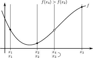
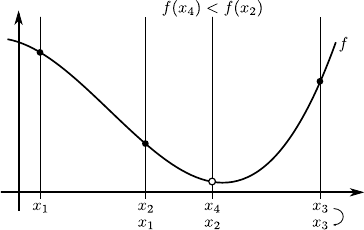
The general principle of the golden section search is to bracket the location of the minimum of .
This is achieved by updating and refining a set of 3 locations
.
The minimization necessarily takes place over a given interval.
The function has to be continuous and unimodal on this interval for the golden section search algorithm to work.
It can be used as the line search procedure for the previously presented algorithm of this section.
It was first proposed in (106) and the refined in (8).
The general principle of the golden section search is to bracket the location of the minimum of .
This is achieved by updating and refining a set of 3 locations
 with the assumptions that
 and
and
 .
These locations are then updated according to the value taken by at a new point
.
These locations are then updated according to the value taken by at a new point  such that
 .
If
.
If
 then the 3 locations become
.
Otherwise, i.e. if
then the 3 locations become
.
Otherwise, i.e. if
 , they become
 .
The principle is illustrated in figure 2.9.
.
The principle is illustrated in figure 2.9.
As just described, the update of the 3 locations implies that the minimum of a function will be located either in the interval
![$ [x_1,x_4]$](img315.png) or
or
![$ [x_2,x_3]$](img316.png) .
The principle of the golden section search algorithm is to impose the length of these two intervals: they must be equal.
It implies that we must have:
.
The principle of the golden section search algorithm is to impose the length of these two intervals: they must be equal.
It implies that we must have:
 |
(2.69) |
where  is the golden ratio, i.e.
 .
.
Contributions to Parametric Image Registration and 3D Surface Reconstruction (Ph.D. dissertation, November 2010) - Florent Brunet
Webpage generated on July 2011
PDF version (11 Mo)