Subsections
Experimental Results
Experiments on Synthetic Data
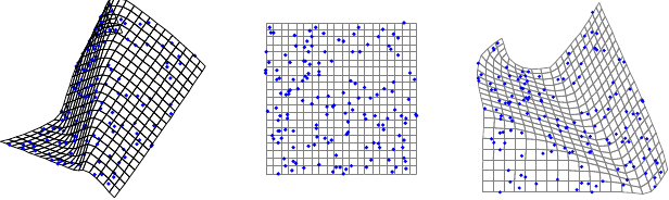
In this section, we experiment several aspects of different reconstruction
algorithms. We first use synthetic piece of papers, such as those of
figure 7.2, randomly generated using the code provided
by (142). The piece of papers are square and 200mm wide. The
input images are simulated by projecting the deformed piece of paper with a
virtual camera placed at approximately 1 meter of the paper sheet and with a
focal length of 36mm. A set of  point correspondences are generated by
taking random locations on the 3D surface. A zero mean Gaussian noise with
standard deviation of 1 pixel is added to the point correspondences. There
are no self-occlusion in the data.
point correspondences are generated by
taking random locations on the 3D surface. A zero mean Gaussian noise with
standard deviation of 1 pixel is added to the point correspondences. There
are no self-occlusion in the data.
Figure 7.2:
Example of randomly generated piece of paper. Left: 3D surface.
Middle: template image. Right: input image. The blue dots are examples
of point correspondences.
|
 |
Several algorithms are compared in our experiments:
- SOCPimg: our point-wise method described in section 7.3.2;
- FFDref: our smooth reconstruction algorithm described in section 7.4.2;
- FFDinit: the initial solution of our smooth reconstruction algorithm, as
described in section 7.4.2;
- Salz: the convex formulation proposed in (166). This method is
similar to SOCPimg except for the noise that
is not handled the same way. In (166), the author minimizes a cost
function that includes a `reprojection error' in order to cope with the noise.
In SOCPimg, the noise is handled with hard constraints.
- PerrioInit: the `upper depth bound' approach
of (143,144) which is a point-wise algorithm that
iteratively enforces the inextensibility constraints ;
- PerrioRef: the `refined approach' of (143,144) which
minimizes a cost function resulting in a refined estimation of the 3D points
obtained with PerrioInit.
The discrepancy between the reconstructed and the ground truth surfaces are
quantified with two measures, depending on the surface model used by the
algorithms. The point-wise reconstruction error (PWRE), denoted  ,
can be used for all the algorithms. It is defined by:
,
can be used for all the algorithms. It is defined by:
 |
(7.16) |
For algorithms that uses more complex surface models, such as triangular meshes
or FFD, we measures the surface reconstruction error (SRE),
denoted  . It is the difference between the reconstructed surface
 and
the ground truth surface
and
the ground truth surface
 :
:
 |
(7.17) |
In this experiment, we use  randomly generated
paper sheets with 150 points
correspondences.
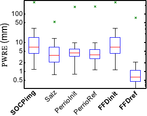
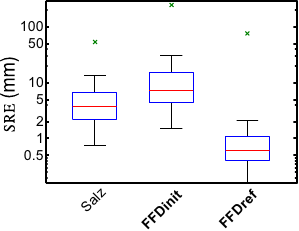
Figure 7.3 (a) shows the PWRE for all the algorithms and
figure 7.3 (b) shows the SRE for the algorithms that use a
complex surface model. The main result of this experiment is that our approach
FFDref gives the smallest reconstruction errors (PWRE and SRE). Globally, the
methods that use complex surface models get better results than the point-wise
approaches.
randomly generated
paper sheets with 150 points
correspondences.
Figure 7.3 (a) shows the PWRE for all the algorithms and
figure 7.3 (b) shows the SRE for the algorithms that use a
complex surface model. The main result of this experiment is that our approach
FFDref gives the smallest reconstruction errors (PWRE and SRE). Globally, the
methods that use complex surface models get better results than the point-wise
approaches.
Figure 7.3:
Comparison of the reconstruction errors for different algorithms. The
central red line is the median. The limits of the blue box are the 25th and the
75th percentiles. The black `whiskers' cover approximately 99.3% of the
experiment outcomes. The green crosses are the maximal errors over the 1000
trials.
|
 |
|
 |
| (a) Point-wise reconstruction error |
|
(b) Surface reconstruction
error |
|
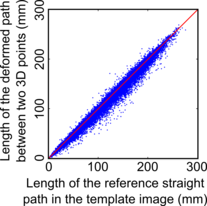
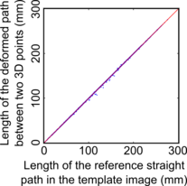
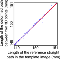
When a reconstructed 3D surface is
reconstructed in a truly inextensible way, the transformation of the
straight line linking two points in the template image must be the geodesic
linking the corresponding two 3D points on the surface. In particular, the
length of these two paths must be identical. Testing this hypothesis for our
algorithms FFDinit and FFDref is the goal of this experiment. To do so, we use the same
data than in the previous experiment. For each surface, we choose randomly
 pairs of points in the template image. For each pair of points
 , the length
 of the deformed path linking the 3D
points
of the deformed path linking the 3D
points
 and
and
 on the surface is
approximated with the following formula:
on the surface is
approximated with the following formula:
 |
(7.18) |
where  is the number of intermediate points used for the approximation (we
use
is the number of intermediate points used for the approximation (we
use  since we experimentally observed that the approximation stabilizes
for values of greater than 180). The lengths of the deformed paths are
plotted against their reference length in the template image in
figure 7.4 (a) for FFDinit and in
figure 7.4 (b,c) for FFDref. Figure 7.4 (b)
and figure 7.4 (c) show that, with the surfaces reconstructed with
FFDref, the length of the deformed paths are almost equal to the length they should
have if they were actual geodesics. In other words, our approach FFDref
reconstructs 3D surfaces which are truly inextensible. On the other hand,
figure 7.4 (a) shows that the initial solution FFDinit (which is
just an FFD fitted to a sparse set of reconstructed 3D points) seems to be much
less inextensible.
since we experimentally observed that the approximation stabilizes
for values of greater than 180). The lengths of the deformed paths are
plotted against their reference length in the template image in
figure 7.4 (a) for FFDinit and in
figure 7.4 (b,c) for FFDref. Figure 7.4 (b)
and figure 7.4 (c) show that, with the surfaces reconstructed with
FFDref, the length of the deformed paths are almost equal to the length they should
have if they were actual geodesics. In other words, our approach FFDref
reconstructs 3D surfaces which are truly inextensible. On the other hand,
figure 7.4 (a) shows that the initial solution FFDinit (which is
just an FFD fitted to a sparse set of reconstructed 3D points) seems to be much
less inextensible.
Let
 be the Euclidean distance between the points
 and
and
 . Table 7.2 gives some statistics on the
relative error between the computed length
and the reference
length
, i.e. the quantity
. Table 7.2 gives some statistics on the
relative error between the computed length
and the reference
length
, i.e. the quantity
 . These numbers confirm the results seen in
figure 7.4.
. These numbers confirm the results seen in
figure 7.4.
The Gaussian curvature is the product of the
two principal curvature (which are the reciprocal of the radius of the
osculating circle). For an inextensible surface, the Gaussian curvature is null.
In this experiment, we check if this property is satisfied by the smooth surfaces
reconstructed with FFDinit and FFDref. We used the same reconstructed
surfaces than in the previous experiment. The Gaussian curvature,
denoted  , is computed for randomly chosen points on the
surface with the formula
, is computed for randomly chosen points on the
surface with the formula
 ,
where
,
where
 and
and
 are the first and the second fundamental forms of
the parametric surface (86). The results of this experiment are
reported in table 7.3. It shows that, in average, the Gaussian
curvature of the surfaces reconstructed using FFDref are consistently close to 0.
It also shows that FFDref gives Gaussian curvatures which are 100 times smaller
than the ones obtained with FFDinit. These results demonstrate that the surfaces
reconstructed with our approach FFDref are indeed inextensible. Note that this kind
of experiment cannot be achieved if a smooth surface is not available.
are the first and the second fundamental forms of
the parametric surface (86). The results of this experiment are
reported in table 7.3. It shows that, in average, the Gaussian
curvature of the surfaces reconstructed using FFDref are consistently close to 0.
It also shows that FFDref gives Gaussian curvatures which are 100 times smaller
than the ones obtained with FFDinit. These results demonstrate that the surfaces
reconstructed with our approach FFDref are indeed inextensible. Note that this kind
of experiment cannot be achieved if a smooth surface is not available.
Experiments on Real Data
The algorithms used in the synthetic experiments of section 7.5.1 are applied to real data in figure 7.5 and figure 7.6.
These figures shows that our approaches gives good results on real data.
In particular, figure 7.5 shows that our method FFDref outperforms the other approaches in the presence of a self-occlusion.
This comes from the fact that FFDref requires the surface to be inextensible everywhere, even if there are no point correspondences (which is the case on the self-occluded part of the paper sheet).
An accurate stereo reconstruction of the surface in figure 7.6 were available.
We compare in table 7.4 the average 3D errors between the surfaces reconstructed with a monocular approach to the stereo reconstruction.
Again, our method FFDref is the one giving the best results.
Figure 7.5:
Illustration of monocular reconstruction algorithms in the presence of a self-occlusion (the point correspondences were automatically extracted using (74)). Note how our algorithm FFDref is able to recover a reasonable shape for the occluded part.
|
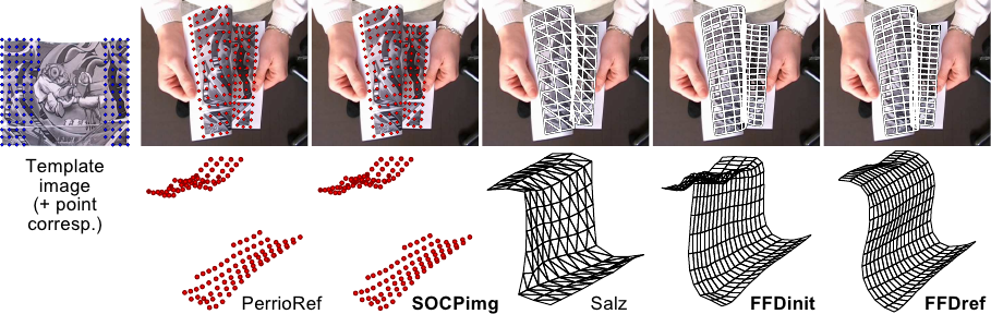 |
Figure 7.6:
Illustration of the results obtained with several monocular reconstruction algorithms. First row: input image along with a reprojection of the reconstructed 3D surface. Second row: reconstructed surface from a different point of view. Note that the stereo reconstruction (first column) is not a monocular algorithm: it is just used to assert the quality of the other reconstructed surfaces (see table 7.4).
|
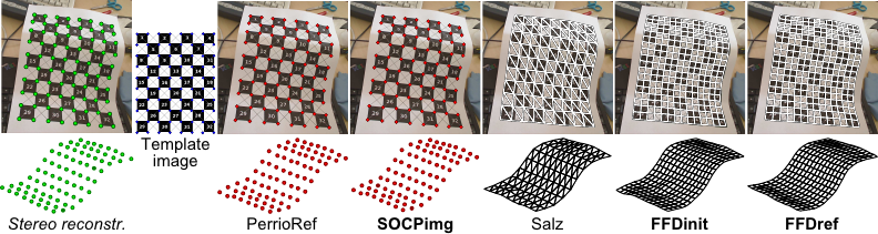 |
Table 7.4:
Average 3D error (in millimeters) with respect to the stereo reconstruction of the surface for the surfaces of figure 7.6.
|
| PerrioRef |
SOCPimg |
Salz |
FFDinit |
FFDref |
|---|
| 2.388 |
2.261 |
4.743 |
2.259 |
1.991 |
|
Contributions to Parametric Image Registration and 3D Surface Reconstruction (Ph.D. dissertation, November 2010) - Florent Brunet
Webpage generated on July 2011
PDF version (11 Mo)