BleamCard: the first augmented reality card. Get your own on Indiegogo!
Subsections
Parametric Models of Function
As it will be seen in the rest of this document, the vast majority of the problems treated in this thesis may be cast into parameter estimation problems.
The fundamental concepts underlying such problems will be detailed in chapter 3.
For now, let us just say that parameter estimation problems consists in finding the parameters of a parametric model so that the resulting function is `close to' a given set of data points.
In a nutshell, a parametric model of function is a function whose exact behaviour is controlled by a set of parameters.
For instance, a polynomial can be considered as a parametric model of function with the polynomial coefficients as parameters.
A more precise definition of the parametric model of function will be given in section 3.1.1.1.
In this section, we detail some particular but generic parametric models of function which are the ones mostly used in this document.
Although we do not pretend to be fully exhaustive, we spend time in explaining the basics on splines and B-splines.
The interested reader can deepen this topic with this readings (61,57,118,67).
We also present other useful parametric models such as rational splines and radial basis functions.
Splines
The word spline is a generic term that designates a parametric model of function.
This word has been used in many contexts (computer aided geometric design, approximation theory, computer vision) with a meaning that slightly varies from one domain to the other.
In this section, we first fix the meaning of the word spline as we understand it in this document.
We then give the basic mathematical definition of a mono-dimensional spline.
We also give the fundamental properties of such objects.
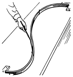
The term spline originally designated a physical object used to draw smooth curves.
It was widely used by engineers and architects to craft blue prints.
It was made of a flexible strip that was fixed at some points.
An illustration of such splines is given in figure 2.10.
Of course, in this document we will be more interested in the mathematical form of the splines than in their physical counterparts.
Figure 2.10:
An historical spline (credits: Pearson Scott Foresman).
|
 |
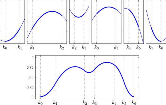
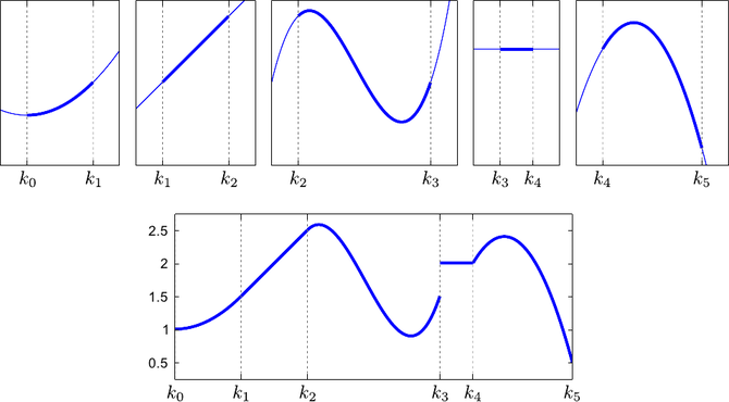
In its most general definition, a spline is a piecewise polynomial function.
Note that this definition is independent of any particular form.
For instance, the B-splines (see section 2.3.2) are just a particular representation of a spline.
Note also that this basic definition does not make any assumption on the continuity of the function.
In particular, the polynomial pieces of a spline may or may not satisfy continuity conditions at their junction.
Examples of splines are given in figure 2.11.
Mathematically speaking, several elements are required to define a spline: a degree, a set of contiguous intervals, and, of course, polynomials on each of this intervals.
The degree of a spline, denoted  in this section, is the maximal degree of the polynomial pieces.
Equivalently, one may talk about the order of the spline, which is
in this section, is the maximal degree of the polynomial pieces.
Equivalently, one may talk about the order of the spline, which is  for a spline of degree .
The intervals are defined using a knot sequence
for a spline of degree .
The intervals are defined using a knot sequence
 which is a strictly increasing sequence of
  real numbers.
The values
real numbers.
The values
 are called the knots.
These knots defines
are called the knots.
These knots defines  knot intervals
![$ [k_i,k_{i+1}]$](img326.png) for
for
 .
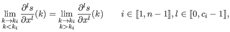
On each knot interval, a spline of degree is defined by a polynomial of degree at most .
The natural definition domain of a spline is the interval
.
On each knot interval, a spline of degree is defined by a polynomial of degree at most .
The natural definition domain of a spline is the interval ![$ [k_0,k_n]$](img328.png) .
For instance, a spline
.
For instance, a spline
![$ s : [k_0,k_n] \rightarrow \mathbb{R}$](img329.png) may be defined as:
may be defined as:
![$\displaystyle s(x) = \sum_{i=0}^d p_{ij} (x - k_j)^i \qquad \begin{cases} \t...
... \llbracket 0,n-2 \rrbracket \textrm{if } x \in [k_{n-1},k_n] \end{cases}$](img330.png) |
(2.70) |
where the values  for
for
 are the coefficients of the
  -th polynomial piece (
 ).
Note that equation (2.70) is just a particular way of expressing a spline.
It is the most basic form for expressing the fact that
).
Note that equation (2.70) is just a particular way of expressing a spline.
It is the most basic form for expressing the fact that  is a piecewise polynomial function.
Other more interesting representations will be given later in this chapter.
is a piecewise polynomial function.
Other more interesting representations will be given later in this chapter.
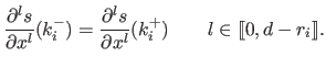
In addition to these basic elements, the polynomial pieces may be stitched to each other using continuity conditions.
These conditions are written:
 |
(2.71) |
where
 is the required class of continuity at the knot
  and where the convention
 is used.
A common choice is
is used.
A common choice is
 .
We name this choice the full continuity constraints.
In this case, the spline belongs to
.
We name this choice the full continuity constraints.
In this case, the spline belongs to
![$ \mathcal{C}^{d-1}([k_0,k_n])$](img340.png) , which is the maximal continuity class for a piecewise polynomial function.
, which is the maximal continuity class for a piecewise polynomial function.
Let us note
 the vector space of the splines of degree with knots
.
Let be a spline of
.
The number of degrees of freedom of the spline is the dimension of the vector space
.
It is the total number of polynomial coefficients minus the number of continuity conditions.
In the full continuity case, the number of degrees of freedom of a spline is
the vector space of the splines of degree with knots
.
Let be a spline of
.
The number of degrees of freedom of the spline is the dimension of the vector space
.
It is the total number of polynomial coefficients minus the number of continuity conditions.
In the full continuity case, the number of degrees of freedom of a spline is
 .
.
A particular way to expressing the splines relies on the truncated power functions.
A truncated power function is denoted with the symbol  .
It is defined as:
.
It is defined as:
 |
(2.72) |
It can be proved (61) that any spline of
can be uniquely written as a linear combination of the canonical monomial  and of the truncated power functions of degree :
 |
(2.73) |
where
 and
and
 are
are  real values.
The polynomials
real values.
The polynomials
 form a basis of the vector space
.
However, this family of functions constitutes an ill-conditioned basis which makes the expression of equation (2.73) numerically unstable.
Therefore, equation (2.73) is not suited for computations.
In the next section, we explore another representation of splines, the so-called B-splines, which is more convenient for practical use.
form a basis of the vector space
.
However, this family of functions constitutes an ill-conditioned basis which makes the expression of equation (2.73) numerically unstable.
Therefore, equation (2.73) is not suited for computations.
In the next section, we explore another representation of splines, the so-called B-splines, which is more convenient for practical use.
The B-spline Representation
In this section, we give the definitions and the properties of the parametric model mostly used in this thesis: the splines expressed as a linear combination of B-splines.
The B-splines are a set of piecewise polynomial functions that defines a suitable basis for the vector space of the splines (the B in B-spline stands for Basis).
As remarked by (56), they were first introduced in (169,53).
We start this section with the construction and the definitions of the basic building block, i.e. the B-spline functions.
We then give the details on the general representation of splines with the B-splines basis functions.
We end this section with a special case of particular interest: the uniform cubic B-splines.
The B-spline  of degree (order ) with knots
 is defined recursively with the following relation:
These formula are only one way of defining the B-splines.
They are called the Cox de Boor recursion formula.
One may remark from equation (2.74) and equation (2.75) that B-splines are themselves splines.
Here comes a list of the most basic properties of the B-spline functions.
These properties were extensively studied in (57,170).
The B-splines are everywhere positive or null:
 |
(2.76) |
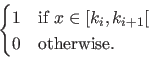
The support of the B-splines is bounded, i.e. they are non-zero only over a their natural definition domain:
![$\displaystyle N_{i,d+1}(x) = 0 \textrm{ if } x \not\in [k_i,k_{i+d+1}]$](img358.png) |
(2.77) |
 |
(2.78) |
For a given degree , the B-splines belongs to the highest possible class of continuity for a piecewise polynomial function:
![$\displaystyle N_{i,d+1} \in \mathcal{C}^{d-1}([k_i,k_{i+d+1}])$](img360.png) |
(2.79) |
The derivative of a B-spline of degree is a linear combination of B-splines of degree  :
:
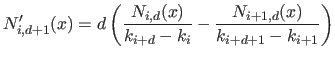 |
(2.80) |
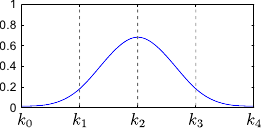
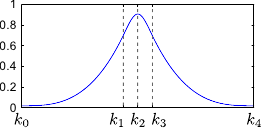
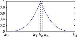
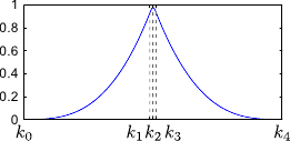
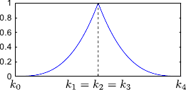
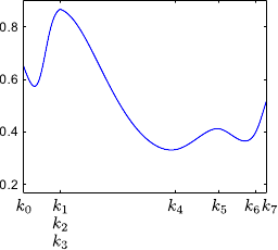
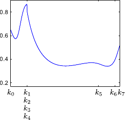
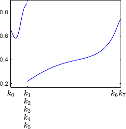
So far, we made the assumptions that the knots were all different.
The definition of the B-splines may be extended to coincident knots.
This allows one to weaken the continuity conditions at the position of these coincident knots.
Let  knots in the set
 be coincident at the point
  (with
(with
 ).
The B-spline have continuous derivatives up to order
).
The B-spline have continuous derivatives up to order  at and is discontinuous at if
  .
Figure 2.12 illustrates the influence of coincident knots on the B-spline basis functions.
.
Figure 2.12 illustrates the influence of coincident knots on the B-spline basis functions.
Let
 be a knot sequence with coincidence allowed.
The break sequence
be a knot sequence with coincidence allowed.
The break sequence
 (with
(with  ) is the strictly increasing sequence of real numbers build by removing the redundancies from the knot sequence:
 |
(2.81) |
The multiplicity of the breaks  is the number of knots that corresponds to the break .
It is denoted with the operator
is the number of knots that corresponds to the break .
It is denoted with the operator
 .
For instance, in equation (2.81), we have that
.
For instance, in equation (2.81), we have that
 .
.
Splines can be written as a linear combination of B-splines basis functions.
Such splines are often referred to as B-splines.
This may be a bit confusing but it is shorter than `splines as a linear combination of B-splines'.
We will use this language shortcut in the rest of this document.
The expression `B-spline basis function' will be utilised to distinguish between the splines and the basis functions.
Let us take back the knot sequence we used when we introduced the spline functions (see section 2.3.1):
 2.3.
Since a single B-spline of degree spans knot intervals,
2.3.
Since a single B-spline of degree spans knot intervals,  independent B-splines can be defined using
 .
The vector space
has dimensions.
Therefore, we need
.
The vector space
has dimensions.
Therefore, we need  supplemental B-splines to form a basis of
.
These B-splines may be defined by adding extra knots to the initial knot sequence satisfying the following conditions:
supplemental B-splines to form a basis of
.
These B-splines may be defined by adding extra knots to the initial knot sequence satisfying the following conditions:
 |
(2.82) |
These additional knots are named the boundary knots.
They must satisfy the conditions of equation (2.82) but may be otherwise arbitrary.
There exists some common choice for defining these boundary knots, later reviewed in this document.
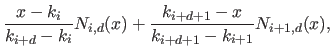
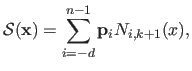
A B-spline is uniquely written as a linear combination of the basis functions for
 :
:
 |
(2.83) |
where the real values  (
) are named the weights (or the coefficients) of the B-spline.
For vector-valued splines (see after), the entities that corresponds to the weights will be called the control points.
Note that equation (2.83) will often be written in vector notation:
(
) are named the weights (or the coefficients) of the B-spline.
For vector-valued splines (see after), the entities that corresponds to the weights will be called the control points.
Note that equation (2.83) will often be written in vector notation:
 |
(2.84) |
where
 and
and
 .
.
The dimension of the vector
is reduced with coincident knots.
Indeed, it corresponds to the number  () of break intervals multiplied by the number of polynomial coefficients on each break interval () minus the number of continuity conditions.
This is consistent with the fact that the order of continuity of a spline is reduced at the location of coincident knots.
Indeed, for a break with multiplicity
() of break intervals multiplied by the number of polynomial coefficients on each break interval () minus the number of continuity conditions.
This is consistent with the fact that the order of continuity of a spline is reduced at the location of coincident knots.
Indeed, for a break with multiplicity  , we have
  continuity constraints instead of :
 |
(2.85) |
We now list some basic properties of the B-splines.
From equation (2.82) and equation (2.83), we see that a B-spline can take non-zero values over the interval
![$ ]k_{-d}, k_{n+d}[$](img399.png) .
Therefore, the interval
.
Therefore, the interval
![$ [k_{-d}, k_{n+d}]$](img400.png) , named the full definition domain, seems to be a good candidate for the definition domain of the spline.
This is not always a good choice.
Indeed, if there are no coincident knots, the boundary values of the splines will always be zero.
Besides, for arbitrary knots, some interesting properties of the B-splines will not be satisfied on
, named the full definition domain, seems to be a good candidate for the definition domain of the spline.
This is not always a good choice.
Indeed, if there are no coincident knots, the boundary values of the splines will always be zero.
Besides, for arbitrary knots, some interesting properties of the B-splines will not be satisfied on
 and
and
![$ ]k_{n},k_{n+d}]$](img402.png) .
For instance, it is the case for the property of the partition of unity (see below).
Besides, on the interval , a B-spline is always the combination of exactly non-zero basis functions (except maybe at the knot position or if some weights are zero).
This is not true on
and
.
Consequently, the definition domain is often a more natural choice than
.
We name this interval the natural definition domain.
Besides, it is more consistent with the general definition of a spline, as explained in section 2.3.1.
.
For instance, it is the case for the property of the partition of unity (see below).
Besides, on the interval , a B-spline is always the combination of exactly non-zero basis functions (except maybe at the knot position or if some weights are zero).
This is not true on
and
.
Consequently, the definition domain is often a more natural choice than
.
We name this interval the natural definition domain.
Besides, it is more consistent with the general definition of a spline, as explained in section 2.3.1.
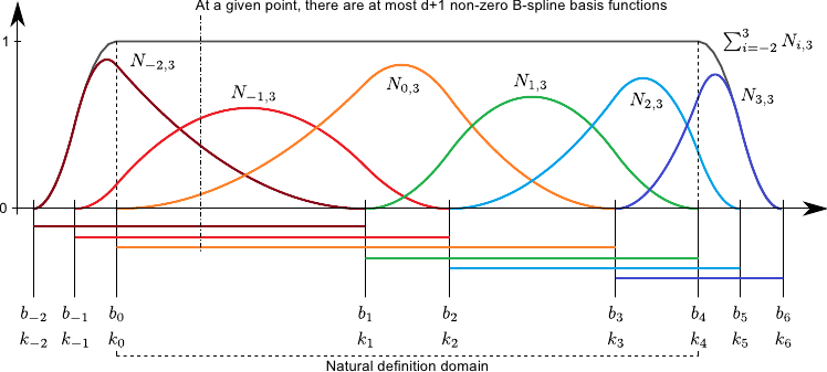
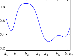
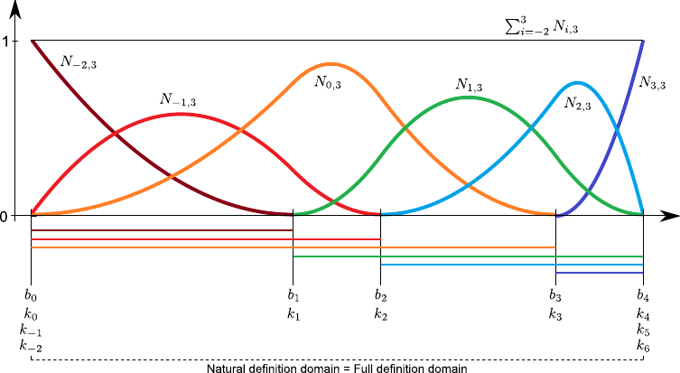
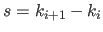
The B-spline basis functions have the interesting property of forming a partition of unity.
This means that we have:
![$\displaystyle \sum_{i=-d}^{n-1} N_{i,d+1} (x) = 1 \qquad \forall x \in [k_0,k_n].$](img403.png) |
(2.86) |
This property is the reason why the B-spline basis functions are often qualified of normalized.
Figure 2.13 illustrates the partition of unity property.
Another interesting property of the B-splines is the fact that the influence of the weights is spatially limited.
This comes from the fact that the B-spline basis functions have a limited support.
Consequently, for a given point  , the value
  is always the linear combination of at most non-zero basis functions.
This is illustrated on figure 2.13.
For reasons that will become clear later in this document, this property allows one to design efficient procedures for parameter estimation with splines.
For now, let us just say that it is obviously faster to compute the sum of numbers than the sum of
is always the linear combination of at most non-zero basis functions.
This is illustrated on figure 2.13.
For reasons that will become clear later in this document, this property allows one to design efficient procedures for parameter estimation with splines.
For now, let us just say that it is obviously faster to compute the sum of numbers than the sum of  numbers (especially when is much more bigger than , which is often the case in practice).
By definition, it is clear that a B-spline is a spline.
Reciprocally, it can also be shown that any spline of
can be represented by a B-spline.
This property is sometimes considered as the fundamental theorem of the B-splines (57).
At this point, the reader who has a minimal background on splines and B-splines might wonder where are the `control points' of the B-spline.
This is generally a confusing point.
As we mentioned earlier, the term `control point' is more conveniently used for vector-valued splines (for instance, a parametric curve embedded in a 2D or 3D space).
In this case, talking about the position of the control points has a meaning (and, besides, some interesting properties can be linked to these positions).
In the mono-dimensional case, and more generally in the scalar-valued case, speaking about the position of the weights does not make much sense.
Indeed, the weight is just a scalar that multiplies the  -th basis function.
It is thus linked to the whole interval on which the basis function is non null (
-th basis function.
It is thus linked to the whole interval on which the basis function is non null (
![$ [k_i,k_{i+d}]$](img407.png) ).
In other words, the weight may be seen as an ordinate without an abscissa.
If one really wants to associate a spatial information to the weight , it might be an horizontal segment of line ranging from to
).
In other words, the weight may be seen as an ordinate without an abscissa.
If one really wants to associate a spatial information to the weight , it might be an horizontal segment of line ranging from to  for the abscissa and of ordinate .
This is illustrated in figure 2.14.
for the abscissa and of ordinate .
This is illustrated in figure 2.14.
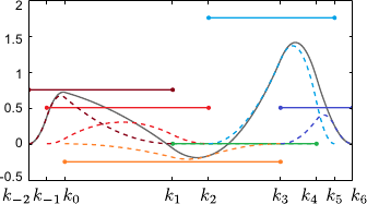
Figure 2.14:
A possible graphical representation of the weights of a mono-dimensional B-spline. In this illustration, we take the same knots and the same degree than in figure 2.13 (in other words, the same B-spline basis functions). The horizontal segments represents the weights applied to each one of the basis functions (the heights are equal to the weights). The dashed curves are the weighted basis functions, i.e. the basis functions multiplied by their corresponding weight. The solid line is the sum of the weighted basis functions, i.e. the final B-spline.
|
 |
Although the expression is not linear with respect to the abscissa , it is linear with respect to the weights.
This is of particular interest in parameter estimation since in such problems we are interested in estimating the weights, not the abscissa.
A linear relation generally leads to easier computations.
Let us temporarily write explicitly the dependency of in the weights
, i.e.
 .
The derivatives of the B-spline with respect to is easily computed:
.
The derivatives of the B-spline with respect to is easily computed:
 |
(2.87) |
Since the derivative of a B-spline basis function of degree is a linear combination of B-spline basis functions of degree (see equation (2.80)), the derivative of a B-spline is a B-spline with one less degree than the original.
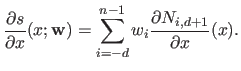
The `derivative', or more precisely the gradient, of with respect to the weights
 is given by:
 |
(2.88) |
The gradient of a spline with respect to the parameters
plays an important role in parameter estimation since it is used by optimization algorithms.
The coincident boundary knots are a common choice for the supplemental boundary knots
 and
and
 .
It is defined by:
.
It is defined by:
 |
(2.89) |
In this case, the full definition domain of the B-spline
coincides with the natural definition domain .
The boundary values of the splines on the full definition domain are not 0 anymore but 1.
Therefore, the partition of unity property is satisfied over the entire definition domain.
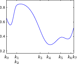
This particular choice of boundary knots is illustrated in figure 2.15.
Note that there exists other choices for the boundary knots.
For instance, one may use arbitrary knots at his convenience or periodic boundary knots (61). This later choice is particularly well suited for approximating periodic functions with B-splines.
We do not detail this choice here because we do not use it in this document.
Figure 2.15:
B-spline with coincident boundary knots. In this case, the partition of unity property is satisfied over all the full definition domain which is the same as the natural definition domain.
|
 |
Uniform Cubic B-Splines
The Uniform Cubic B-Splines (UCBS) are a special case of B-splines which are particularly interesting for their simplicity and efficiency.
As the name indicates, they are B-splines of degree 3.
This degree is a good compromise between flexibility and simplicity of the induced computations.
The word uniform means that all the knots are equally spaced.
In this case, the B-splines basis functions are just shifted copies of each others:
 |
(2.90) |
where is the width of a knot interval (i.e.
 for all
 ).
Figure 2.16 shows a set of B-spline basis functions in the UCBS case.
For the sake of simplicity, we drop the index that indicates the order in the notation of the B-spline basis functions, i.e.
).
Figure 2.16 shows a set of B-spline basis functions in the UCBS case.
For the sake of simplicity, we drop the index that indicates the order in the notation of the B-spline basis functions, i.e.
 .
.
Figure 2.16:
The B-spline basis functions for UCBS are shifted copies of each others. On the natural definition domain (![$ [k_0,k_3]$](img420.png) on this figure), there are always 4 non-zero basis functions.
on this figure), there are always 4 non-zero basis functions.
|
 |
When dealing with UCBS, it is often more convenient to work with normalized abscissa than with original abscissa.
The normalized abscissa consists in scaling and translating the abscissa so that the knot  coincides with 0 and so that the width of the knot intervals equals 1.
Let
coincides with 0 and so that the width of the knot intervals equals 1.
Let
 be the knot sequence.
The normalized abscissa of the point , denoted
be the knot sequence.
The normalized abscissa of the point , denoted  , is defined by:
 |
(2.91) |
where is the original width of a knot interval, i.e.
(
 ).
).
The knot interval in which a point lies is denoted  .
.
 is a function from
![$ [k_{-3}, k_{n+3}]$](img428.png) to
to
 defined as follows:
 |
(2.92) |
The normalized 0-based abscissa of is the number  such that:
 |
(2.93) |
It corresponds to the abscissa of the point in a local coordinate frame so that the lower bound of the knot interval in which the point lies coincides with 0 and of width 1.
A closed form expression of the UCBS basis functions can be computed by unrolling the Cox-de Boor recursive relations that defines the B-spline basis functions (equation (2.74)).
Without loss of generality, we consider that the knot sequence is normalized and 0-based.
If it was not the case, one would just have to replace by in the right-hand side of the following equations.
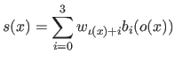
The -th basis function of the UCBS is expressed as:
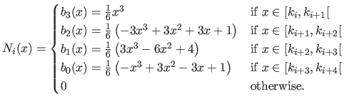 |
(2.94) |
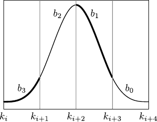
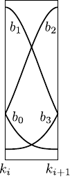
Figure 2.17 gives an illustration of the B-spline basis function for the UCBS.
The evaluation of a B-spline at a point is then equivalent to a blending of the four weights closest to the point .
The blending functions are the four polynomials
 of degree 3 that constitutes the B-spline basis function.
In other words, we have that:
of degree 3 that constitutes the B-spline basis function.
In other words, we have that:
 |
(2.95) |
Figure 2.17:
Anatomy of a B-spline basis function of UCBS. (a) A B-spline basis function of a UCBS is made of four pieces, each one of which being a polynomial of degree 3. (b) On a given knot interval, the value of a B-spline can be viewed as the blending of the four adjacent coefficients of the B-spline with weights given by the basis functions.
|
 |
|
 |
| (a) |
|
(b) |
|
As any B-spline, a UCBS can be written in vector notation:
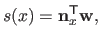 |
(2.96) |
 |
(2.97) |
Remark that the vector
 has at most 4 non-zeros entries, whatever the size of the knot vector (i.e. the number of weights).
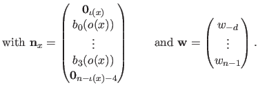
The matrix notation is another common notation for the UCBS.
It explicitly reveals that, on a given knot interval, a UCBS is a polynomial function of degree 3 with coefficients obtained by blending the weights of the 4 non-zero B-spline basis functions that corresponds to this knot interval.
As we will see later in this manuscript, the matrix notation can make easy some computations that would have been more difficult otherwise.
It is given by:
 |
(2.98) |
where  is known as the geometric matrix (118) and is defined by:
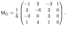 |
(2.99) |
Although we do not use them in this document, other type of splines can be written in the form of equation (2.98) just by changing the geometric matrix.
For instance, this is the case for the cubic Hermite splines (67).
One of the most important application of the splines is to interpolate a sparse set of data point.
Let
 be the data set.
The natural spline is the `least bended' function that interpolates the data set.
It is the solution to the following variational problem:
be the data set.
The natural spline is the `least bended' function that interpolates the data set.
It is the solution to the following variational problem:
 |
(2.100) |
where  is the functional that gives the bending energy of a function over its definition domain
  (here,
![$ \displaystyle \Omega = \big[\min_i x_i, \max_i x_i \big]$](img445.png) ).
It is defined as:
).
It is defined as:
![$\displaystyle B[f] = \int_{\Omega} \left ( \frac{\partial^2 f}{\partial x^2}(x) \right )^2 \mathrm d x$](img446.png) |
(2.101) |
The solution to problem (2.100) is a B-spline of degree 3 with knots identical to the abscissa of the data points (57).
B-Splines in Higher Dimensions
In this section, we extend the B-splines as presented in the previous section to higher dimensions.
Note that for the sake of simplicity, we restrict our study to B-splines although most of the concept presented in this section could be applied to arbitrary splines.
We first show how vector-valued B-splines can be defined.
We will not spend much time on these aspects since they are barely used in the rest of this document.
We then consider a case of greater importance in this thesis: the bivariate B-splines built using the tensor-product of univariate B-splines.
Vector-valued B-splines can easily be constructed from scalar-valued B-splines by replacing the weights with control points.
A vector-valued B-splines
 is thus defined by:
 |
(2.102) |
where the
 are the control points of the B-splines.
They are vector of
are the control points of the B-splines.
They are vector of
 .
With
.
With  , equation (2.102) is the equation of a parametric curve embedded in a plane.
With
, equation (2.102) is the equation of a parametric curve embedded in a plane.
With  , equation (2.102) describes a parametric curve embedded in space.
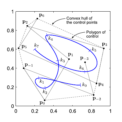
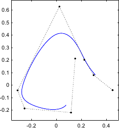
An illustration of vector-valued (with ) is given in Figure 2.18.
, equation (2.102) describes a parametric curve embedded in space.
An illustration of vector-valued (with ) is given in Figure 2.18.
Contrarily to the scalar-valued case, it makes sense to speak about the position of the control points.
While a weight could be seen as an ordinate without an abscissa, a control point
 completely defines a point in dimensions.
Besides, some properties can be attached to the position of the control points.
The set of all the control points
completely defines a point in dimensions.
Besides, some properties can be attached to the position of the control points.
The set of all the control points
 defines what is called the polygon of control.
An interesting property is that the B-spline is always included in the convex hull of the polygon of control
defines what is called the polygon of control.
An interesting property is that the B-spline is always included in the convex hull of the polygon of control  .
.
One of the most simple approach to extend the univariate B-splines to two variables is known as the tensor product B-spline.
The use of the expression tensor product will become clear later as we will see that it is related to the tensor product of two matrices (also known as the Kronecker product).
We restrict our study of the tensor product splines to the case of two variables but the same principles could be applied for higher dimensions (but with a dramatic increase in the notation burden).
Let
 and
and
 be two knot sequences.
The (scalar-valued bivariate) tensor product B-spline of degree
be two knot sequences.
The (scalar-valued bivariate) tensor product B-spline of degree  along the -direction and
  along the
  -direction is the function from
![$ [k_0,k_{n_x}] \times [l_0,l_{n_y}]$](img465.png) 2.4 to
2.4 to
 defined as:
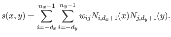 |
(2.103) |
The main advantage of the tensor product approach is that most of the properties of the univariate B-splines are still true in the bivariate case.
This is true, for instance, for the partition of unity property, or for the local support of the basis functions.
The definition of equation (2.103) can be interpreted in different ways.
We give two of these interpretations in the next two paragraphs.
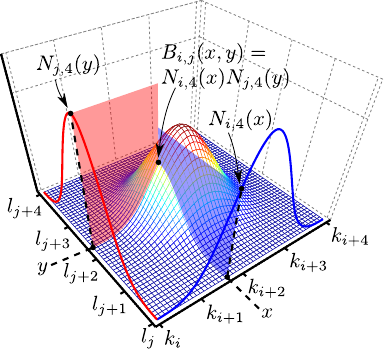
One can consider the tensor product B-splines as a linear combination of the bivariate basis functions  (for
(for
 and
and
 ) which are bivariate polynomials of degree in and in defined as:
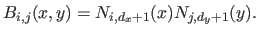 |
(2.104) |
Given the properties of the univariate B-spline basis functions, the basis function is non-zero only over the interval
![$ [k_i,k_{i+d_x+1}] \times [l_j,l_{j+d_y+1}]$](img472.png) .
The construction of the tensor product B-spline basis functions is illustrated in figure 2.19.
.
The construction of the tensor product B-spline basis functions is illustrated in figure 2.19.
On a sub-domain
, a univariate spline of degree is a single polynomial of degree .
This can be written in vector form as follows:
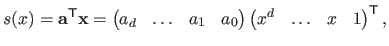 |
(2.105) |
where the values
 are the coefficients of the polynomial.
On a sub-rectangle
are the coefficients of the polynomial.
On a sub-rectangle
![$ [k_i,k_{i+1}] \times [l_j,l_{j+1}]$](img479.png) , a tensor product spline is given by the tensor (or Kronecker) product of a polynomial of degree in and in .
Let
, a tensor product spline is given by the tensor (or Kronecker) product of a polynomial of degree in and in .
Let  and
and  be those two polynomials:
The fact that a tensor product spline is the tensor product of two univariate polynomial can be seen from the following identity:
 |
(2.108) |
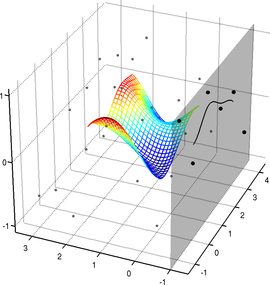
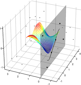
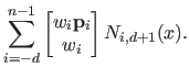
Another common way of interpreting the basic definition of equation (2.103) of the tensor product B-spline is to see that each `slice' parallel to the -axis of the surface is a univariate spline with weights that are themselves defined by B-splines.
It can be seen by rearranging equation (2.103) as follows:
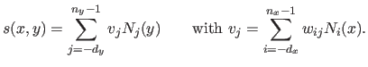 |
(2.109) |
This point of view is illustrated in figure 2.20.
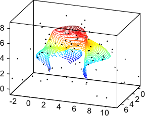
The extensions of the B-splines to the vector-valued bivariate case can be combined.
In particular, this allows one to define parametric surfaces embedded in a 3D space, which is a function from
 to
to
 .
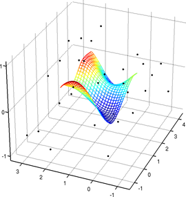
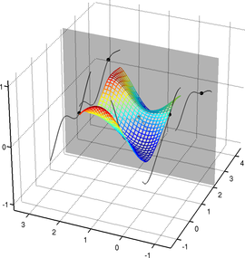
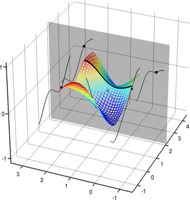
An example of such surface is presented in figure 2.21.
We will make use of this type of surface model for the NURBS-Warps and for the monocular reconstruction of inextensible surfaces.
.
An example of such surface is presented in figure 2.21.
We will make use of this type of surface model for the NURBS-Warps and for the monocular reconstruction of inextensible surfaces.
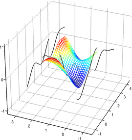
Figure 2.21:
Example of a parametric surface described with a 3-vector-valued tensor-product B-spline.
|
 |
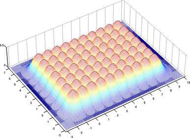
As in the univariate case, bivariate tensor-product B-splines of degree 3 defined with the help of uniformly distributed knot sequences are of particular interest.
Indeed, such B-splines involves only polynomials of degree 3 which make the computations more stable.
Besides, these computations are simplified in the sense that the bivariate basis functions are shifted copies of each other, as illustrated in figure 2.22.
This type of tensor product B-spline is also abbreviated UCBS.
Figure 2.22:
The bivariate tensor product B-spline basis functions for UCBS are shifted copies of each others. Here the full definition domain is represented, i.e.
![$ [k_{-3}, k_{10}] \times [l_{-3},l_{7}]$](img495.png) .
.
|
 |
Non Uniform Rational B-Splines (NURBS)
The rational splines are another parametric model of function that will be used in this document.
As the name may indicate, this model is defined as the ratio of two splines.
Rational splines are particularly interesting in computer vision since they may be seen as the perspective projection of standard splines.
Although any type of spline could be used, we focus on a particular type of rational splines that relies on B-splines: the Non-Uniform Rational B-Splines (NURBS).
We first give the definition of a univariate scalar-valued NURBS.
Let
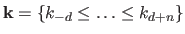 be a knot sequence, with the degree of the NURBS.
A NURBS is a function model parametrized by points
be a knot sequence, with the degree of the NURBS.
A NURBS is a function model parametrized by points  (
)), each one of those associated to a strictly positive2.5 weight .
Let
(
)), each one of those associated to a strictly positive2.5 weight .
Let
![$ r : [k_0,k_n] \rightarrow \mathbb{R}$](img498.png) be the NURBS.
Its expression is given by (42,67):
be the NURBS.
Its expression is given by (42,67):
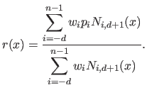 |
(2.110) |
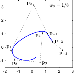
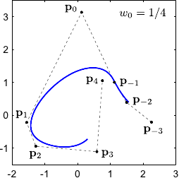
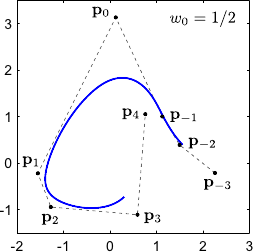
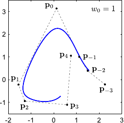
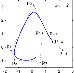
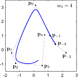
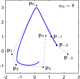
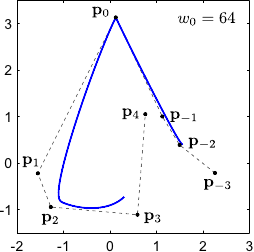
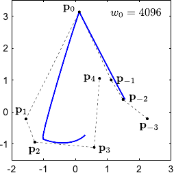
The weight controls the influence of the point .
In particular, the bigger the closer to the NURBS.
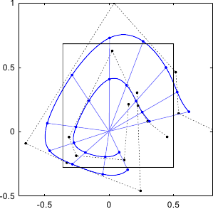
This property is illustrated on figure 2.23 for 2-vector-valued NURBS.
Another common writing of the NURBS consists in expressing them as a combination of basis functions with the control points as the coefficients:
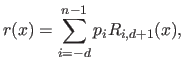 |
(2.111) |
where  is the -th rational basis function of degree (order ):
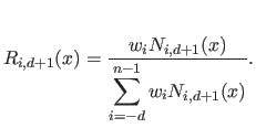 |
(2.112) |
Although the writing of equation (2.111) seems similar to the definition of the B-splines, it is in fact quite different.
Indeed, the B-spline basis functions were functions independent of the parameters of the B-spline.
On the contrary, the rational basis functions depend on the weights of the NURBS.
Consequently, the NURBS are not linear with respect to the parameters.
Even if the concepts behind the rational basis functions and the B-spline basis functions are different, they still share some properties.
This will be reviewed and illustrated in the paragraph dedicated to the properties of the NURBS.
As for the B-splines, the NURBS can be generalized to higher dimensions.
An -vector-valued NURBS is obtained from equation (2.110) by replacing the scalars by vectors
.
The weights remain unchanged and they still control the influence of the control points
.
Multi-variate NURBS are derived from equation (2.110) using tensor product B-splines for both the numerator and the denominator.
For instance, given two knot sequences
and
, a 3-vector-valued bivariate NURBS (i.e. a parametric surface embedded in a 3D space) is the function
 from
to
defined by:
from
to
defined by:
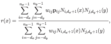 |
(2.113) |
with
 and
and
 for all
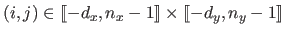 .
.
Figure 2.23:
Influence of the weights associated to the control points of a 2-vector-valued NURBS.
|
|
Let
be an -vector-valued univariate NURBS.
One may notice that the vector
 are the Cartesian coordinates of the following point expressed in homogeneous coordinates:
 |
(2.114) |
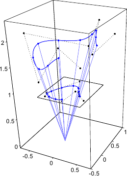
Equation (2.114) is the exact definition of an  -vector-valued B-spline.
In other words, an -vector-valued NURBS is the perspective projection of an -vector-valued B-spline.
This fact is illustrated in figure 2.24.
-vector-valued B-spline.
In other words, an -vector-valued NURBS is the perspective projection of an -vector-valued B-spline.
This fact is illustrated in figure 2.24.
The NURBS share many properties with the B-splines.
In addition, they have supplemental interesting properties.
We now give a brief overview of these properties.
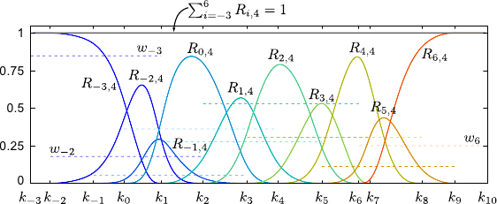
As for the B-splines, the rational basis functions form a partition of unity, i.e. :
![$\displaystyle \sum_{i=-d}^{n-1} R_{i,d+1}(x) = 1 \qquad \forall x \in [k_{-d}, k_{n+d}].$](img512.png) |
(2.115) |
Note that this property hold true for any set of weights.
Figure 2.25 illustrates this property.
Note also that for B-splines this property was satisfied only over the natural definition domain.
For NURBS, it is satisfied over all the full definition domain.
This comes from the fact that the rational basis function are normalized and, therefore, the rightmost (and the leftmost) basis functions does not vanish to zero.
The rational basis functions have a compact support:
![$\displaystyle R_{i,d+1}(x) = 0 \qquad \forall x \not\in [k_i,k_{i+d+1}].$](img514.png) |
(2.116) |
In other word, the -th control point and the -th weight influences the shape of the resulting NURBS only over the knot intervals
![$ [k_i,k_{i+d+1}]$](img515.png) .
.
NURBS have continuous derivatives up to order .
In other words, we have that:
![$\displaystyle r \in \mathcal{C}^d([k_{-d}, k_{d+n}]).$](img516.png) |
(2.117) |
As with the B-splines, it is possible to diminish these continuity conditions at the position of the knots by using multiple knots.
This is illustrated in figure 2.26.
Several `types' of derivatives are useful for parameter estimation: with respect to the free variable , to the control points
 , and to the weights
 .
In this paragraph, we will write explicitly the dependency of in all its parameters, i.e.
.
In this paragraph, we will write explicitly the dependency of in all its parameters, i.e.
 .
For the sake of simplicity, let us note and the numerator and the denominator of :
.
For the sake of simplicity, let us note and the numerator and the denominator of :
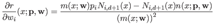
We just give the formula of the different derivatives.
More detailed computations can be found in (42).
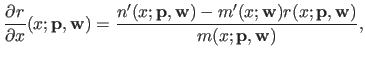 |
(2.120) |
where  and
and  denote the derivatives of and with respect to .
The gradient of with respect to
 is given by:
 |
(2.121) |
where the functions (
) are the rational basis functions defined in equation (2.112).
The gradient of with respect to
is given by:
 |
(2.122) |
with
 |
(2.123) |
Although we will not need this property in this document, it is still worth noticing that conic sections can be represented with NURBS.
It is an ability that standard splines, in particular B-splines, do not have.
Splines can only approximate conic sections.
We will not give the details underlying the representation of conics with NURBS (which can be found in, for instance, (118)).
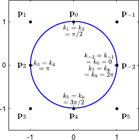
We just give a classic example in figure 2.27: the representation of a circle.
Figure 2.27:
Exact representation of a circle with a NURBS of degree 2. Standard splines such as B-splines can only approximate a conic, not represent them exactly.
|
 |
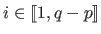
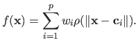
Radial Basis Functions (RBF) are another model of parametric functions.
Let
 be an RBF.
The function
be an RBF.
The function  is of the following form:
 |
(2.124) |
The real values (
 ) are the weights of the RBF.
They can be vectors of
in which case the RBF is a function from
) are the weights of the RBF.
They can be vectors of
in which case the RBF is a function from
 to
.
The second term in equation (2.124) is the affine part where the functions
to
.
The second term in equation (2.124) is the affine part where the functions  (
(
 ) are monomials of order up to 1 (156).
The vectors
) are monomials of order up to 1 (156).
The vectors
 (
(
 ) are called the centres of the RBF.
They are generally fixed values, i.e. they are not part of the parameters to be estimated in a parameter estimation problem.
Broadly speaking, the centres define the number of degrees of freedom of the RBF.
Finally,
) are called the centres of the RBF.
They are generally fixed values, i.e. they are not part of the parameters to be estimated in a parameter estimation problem.
Broadly speaking, the centres define the number of degrees of freedom of the RBF.
Finally,  is a function from
 to
.
It is the basis function of the RBF.
The norm
to
.
It is the basis function of the RBF.
The norm
 in equation (2.124) is not necessarily the Euclidean norm ; it can be any norm.
Common basis functions will be given in section 2.3.4.2.
Contrarily to the spline model, the RBF are naturally designed as multi-variate functions.
This can be an advantage compared to the splines because the tensor-product approach used with splines to handle multi-variate functions has some limitations.
in equation (2.124) is not necessarily the Euclidean norm ; it can be any norm.
Common basis functions will be given in section 2.3.4.2.
Contrarily to the spline model, the RBF are naturally designed as multi-variate functions.
This can be an advantage compared to the splines because the tensor-product approach used with splines to handle multi-variate functions has some limitations.
Note that under some assumptions, the affine part in equation (2.124) can be dropped.
The RBF thus becomes:
 |
(2.125) |
Since an RBF is linear with respect to its weights, it can be written in vector form:
 |
(2.126) |
where
 and
are two vectors of
and
are two vectors of
 that are defined in the following way:
Note that the vector
may depend on
 in a nonlinear fashion.
However, this does not change the fact that an RBF is linear with respect to the weights
.
Note also that RBF are very similar to splines in the sense that they are both a linear combination of basis functions.
The differences are the form of the basis functions and their locations.
in a nonlinear fashion.
However, this does not change the fact that an RBF is linear with respect to the weights
.
Note also that RBF are very similar to splines in the sense that they are both a linear combination of basis functions.
The differences are the form of the basis functions and their locations.
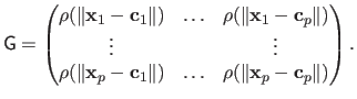
For reasons that will become clear later in this document, the Gram matrix (54) plays an important role in parameter estimation problems with RBF.
Let
 be a set of vectors, the number of which being identical to the number of centres of the RBF.
The Gram matrix is the matrix
be a set of vectors, the number of which being identical to the number of centres of the RBF.
The Gram matrix is the matrix
 defined as follows:
 |
(2.129) |
For now, let us just say that parameter estimation problems with RBF involves the inversion of the matrix
 .
Therefore, the definiteness of the Gram matrix is an important property.
The definiteness of the Gram matrix depends on the basis function .
.
Therefore, the definiteness of the Gram matrix is an important property.
The definiteness of the Gram matrix depends on the basis function .
Basis Functions
In this section, we give details on classical basis functions for RBF (152).
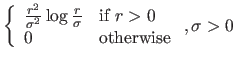
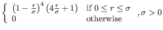
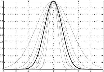
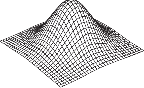
Table 2.2 gives the expression and some basic properties of common basis functions for RBF.
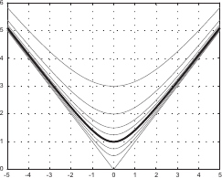
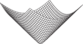
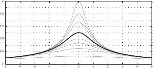
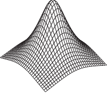
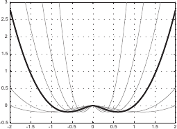
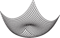
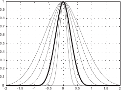
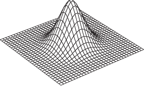
These basis functions are illustrated in figure 2.28 in the univariate and the bivariate cases.
Among the basis functions described in table 2.2, two are of particular interest in computer vision: the Thin-Plate Spline (TPS) basis functions and the Wendland's basis functions.
The TPS are sometimes considered as the natural extension to the bivariate case of the cubic B-splines (193).
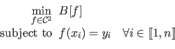
This comes from the fact that these two models are the functions that minimizes the following variational minimization problem:
![$\displaystyle \min_{f : \mathbb{R}^n \rightarrow \mathbb{R}} B[f],$](img559.png) |
(2.130) |
with  in the cubic B-spline case and
  in the TPS case.
The functional is the bending energy.
If
in the TPS case.
The functional is the bending energy.
If  , it is defined as:
![$\displaystyle B[f] = \iint_{\mathbb{R}^2} \left ( \frac{\partial^2 f}{\partial ...
... + \left ( \frac{\partial^2 f}{\partial y^2} \right )^2 \mathrm d x \mathrm d y$](img563.png) |
(2.131) |
TPS have been widely used in computer vision (11,62,24,18).
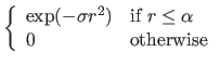
The Wendland's basis functions are another type of basis functions that are particularly interesting for several reasons (73).
First, they are expressed as polynomials of relatively low order, which makes them easier to compute than basis functions relying on `exotic' functions such as the logarithm or the exponential.
Second, the Wendland's basis function have a bounded support.
It means that the influence of a weight is spatially limited.
This is not the case with, for instance, the TPS.
Contributions to Parametric Image Registration and 3D Surface Reconstruction (Ph.D. dissertation, November 2010) - Florent Brunet
Webpage generated on July 2011
PDF version (11 Mo)